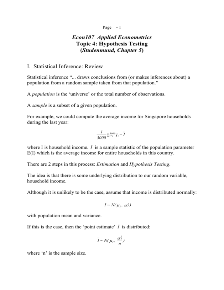
Page
-1
Econ107 Applied Econometrics
Topic 4: Hypothesis Testing
(Studenmund, Chapter 5)
I. Statistical Inference: Review
Statistical inference “... draws conclusions from (or makes inferences about) a
population from a random sample taken from that population.”
A population is the ‘universe’ or the total number of observations.
A sample is a subset of a given population.
For example, we could compute the average income for Singapore households
during the last year:
1
3000
i=1 I i = I
3000
where I is household income. I is a sample statistic of the population parameter
E(I) which is the average income for entire households in this country.
There are 2 steps in this process: Estimation and Hypothesis Testing.
The idea is that there is some underlying distribution to our random variable,
household income.
Although it is unlikely to be the case, assume that income is distributed normally:
I ~ N(  I ,  2I )
with population mean and variance.
If this is the case, then the ‘point estimate’ I is distributed:
I ~ N(  I ,
where ‘n’ is the sample size.
 2I )
n
Page
-2
Which we can turn into a ‘standardized’ normal distribution by subtracting the
population mean and dividing by the standard deviation of the estimator.
Z=
I - I
I / n
~ N(0, 1)
Of course, we don’t know the population standard deviation σI, but we can replace
it with the sample standard deviation (S):
̂ = S =
1
2
n
 i=1 ( I i - I )
n -1
and rewrite the earlier expression:
t=
I - I
S/
n
which follows a t distribution with (n-1) degrees of freedom.
We can look up the critical t values in the Table for the t-distribution:
Prob(-2.576  t  2.576) = 0.99
Substitute in the earlier expression for t and rearrange terms:
Prob( I -
2.576 S
n
 I  I +
2.576 S
n
) = 0.99
This is the Confidence Interval around the unknown population parameter μI.
Interpretation: there is a 99% probability that this ‘random interval’ contains the
true μI. Confidence level=100%-Significance level.
Suppose I = 40 (i.e., the average household receives $40,000 per year), and the
sample standard deviation is 10.
40 -
25.76
25.76
  I  40 +
=
54.772
54.772
39.530   I  40.470
Page
-3
Properties of Point Estimators
•
Linearity. An estimator is linear if it’s a linear function of the observations
in the sample.
I=
•
1
1
3000
( I1 + I 2 + ... + I n )
i=1 I i =
3000
3000
Unbiasedness. An estimator is unbiased if in repeated samples the mean
value of the estimators is equal to the true parameter value.
E( I ) =  I
•
Efficiency. This has to do with the ‘precision’ of our estimator. An
estimator is efficient if it has the smallest variance among other linear
unbiased estimators. It’s BLUE (Best Linear Unbiased Estimator).
•
Consistency. An estimator is ‘consistent’ if it approaches the true
parameter value as the sample size gets larger.
Note that the properties of unbiasedness and consistency are conceptually very
different. Unbiasedness can hold for any sample size. Consistency is strictly a
large-sample property.
Suppose we want to ‘test the hypothesis’ that the true mean income of households
is equal to some value. For example, we might test the null hypothesis that it’s
equal to $41,000.
H 0 :  I = 41.0
H 1 :  I  41.0
This is known as a two-sided alternative hypothesis. An example of a one-sided
alternative hypothesis is that this true parameter is greater than $41K.
II. Three Typical Approaches to Hypothesis Testing: Review.
1. The Interval Approach.
We computed earlier the 99% confidence interval for μI.
39.530   I  40.470
Page
-4
Therefore, if a particular null hypothesis doesn’t lie within this interval, we can
reject it. The confidence interval is also known as the Acceptance Region. If not
within this interval, it lies in the Rejection Region.
Might want to say something about the different ‘types’ of mistakes that one can
make in these hypothesis tests.
•
‘Type I’ Error. Rejecting a null hypothesis when it’s true. Not always
going to be right.
Type I Error = Prob(Rejecting H0 | H0 is True) = α.
where this is a ‘conditional probability’, and α is .01. This is the
‘significance level’ chosen.
•
‘Type II’ Error. Accepting a null hypothesis when it’s false. Suppose our
null had been that the mean household income was $40,250. This clearly
lies with the confidence interval. We’d not reject the null. Yet, the truth is
it might be $41,000.
Type II Error = Prob(Accepting H0 | H0 is False) = β.
This probability has been traditionally assigned the Greek letter β (do not confuse
this β with β’s used in the regression model). One minus this value is called the
Power of the Test. The classical approach is to set α to be a small number and
minimise β (or maximise the power of the test given the confidence level).
2. The Significance Test Approach.
We know that the statistic computed from the sample follows a t distribution with
n-1 degrees of freedom.
t
I  I
S/ n
Let’s take the earlier example. Suppose we want to know whether or not μI is
equal to 41.
t=
40 - 41
 - 5.477
10 / 3000
Page
-5
Can we reject the null? Depends on the confidence level. Suppose again that we
set α=.01. Again, it’s a two-sided test.
Pr ob(| t | 2.576)  0.01
Clearly, the absolute value of our computed t exceeds this critical value. We reject
the null that the true mean household income is $41,000.
What about another null, for example that the population mean is equal to $40,250?
Compute the t statistic as:
t=
40 - 40.25
 - 1.369
10 / 3000
Clearly, here we’d be unable to reject this null.
In econometrics, more often than not, we test the null that the estimator is equal to
zero. In other words, whether or not an estimated coefficient is significantly
different from zero. The terminology is that the estimated coefficient is
‘statistically significant’. In context of this example, this is written:
t=
I
S / n
where the numerator is the estimated coefficient and the denominator is the
estimated standard error.
3. The ‘P Value’
The problem with classical hypothesis testing is that one has to choose a particular
significance level. This is quite arbitrary. Conventionally, α is set equal to 0.10,
0.05 and/or 0.01.
The way around this is to compute the Exact Significance Level or P Value. This
is the largest significance level at which the null cannot be rejected (or the lowest
significance level at which the null can be rejected). Consider the earlier example.
Instead of specifying α and looking up the critical value, you plug in the computed
t statistic as the critical value and ‘look up’ the corresponding α.
Page
-6
Prob( | t | > 5.477) = .0001
In this case, 5.477 is ‘just significant’ at a .01% level.
A more typical result might be the following:
Prob( | t | > 2.196) = .0355
This says that this test is significant at a 3.55% level. At 5%, the null is rejected,
but at the 1% level, we cannot reject the null.
Inference about the population variance:
The sample variance S 2 is an unbiased, consistent and efficient point estimator
for  . The statistic
2
(n  1) S 2
2
has a distribution called Chi-square with (n-1)
degrees of freedom, if the population is normally distributed.
Inference about the ratio of two population variances:
The parameter to be tested is  12 /  22 . The statistic used is
S12 /  12
which has a
S 22 /  22
distribution called F with degrees of freedom being n1  1 and n2  1, if the two
populations are normally distributed.
III. Hypothesis Testing in Linear Regression Models
Suppose we want to test the hypothesis in linear regression models,
H 0 : 1 = 0
H 1 : 1  0
Why is the test important? How to test it? Note that we typically put the value(s)
that we do not expect in the null hypothesis and put the values that we expect to
be true in the alternative hypothesis.
We note that
ˆ
where Var( ̂ 1 ) =  2 .
2
 xi
1
~ N(  , Var ( ˆ ) )
1
1
Page
-7
So by standardisation, we have
ˆ1  1
~ N (0,1)
 ( ˆ1 )
We can use this sampling distribution to make statistical inferences. However,
when the standard deviation of OLS estimator is unknown, this sampling
distribution is not applicable. We can substitute sigma by its estimator and get a
new statistic (with a new sampling distribution)
ˆ1 -  1 ( ˆ1 -  1 )  xi2
t=
=
~ t ( n K 1)
ˆ
s( ˆ1 )
where s( ˆ1 ) =
ˆ
 xi
2
(in SLRM), K is the number of independent variables. This
is a t distribution with n-K-1 degrees of freedom.
We’ve gone through the ‘general mechanics’ already, so let’s use a specific
numerical example to see how we would proceed. To illustrate, suppose we want
to put a ‘confidence interval’ around  1 and suppose we had a cross section of 10
households, and we wanted to estimate our linear consumption function. We get
the following:
Cˆ = 24.455 + .509 DI i
(6.414) (.036)
n = 10 df = 8 ̂ 2 = 42.159 R 2 = .962
We want to place a confidence interval around the estimated slope coefficient.
Need to choose a confidence level. Suppose 95% (α=.05). Two-tailed test. Look
it up in the table. Critical value is 2.306. Now recall the general expression for the
confidence interval.
Prob[ ˆ1 - t/2 s( ˆ1 )   1  ˆ1  t/2 s(ˆ1 ) ] = 1 - 
.509 - (2.306) (.036)   1  .509 + (2.306) (.036)
.4268   1  .5914
Page
-8
Plugging in the values and estimates from above we get:
Might want to construct the 95% confidence interval for β0. You should get the
following:
9.664   0  39.245
Now suppose I want to perform a two-sided test.
H 0 :  1 = 0.3
H 1 :  1  0.3
We want to know whether or not the true MPC is 0.3, where the alternative
hypothesis is that it’s something other than 0.3. Compute the t statistic from the
general formula above:
t=
.509 - .3
= 5.806
.036
which is significant at better than a 5% level (critical value given above as 2.306),
and 1% level (critical value 3.355). Reject the null.
Page
-9
the density function for the t variable
Now suppose I want to perform a one-sided test.
H 0 :  1  0.4
H 1 : 1 > 0.4
We want to know whether or not the true MPC is less than or equal to 0.4, where
the alternative hypothesis is that it’s greater than 0.4.
Compute the t statistic:
t=
.509 - .4
= 3.028
.036
but note that the formula and procedure are identical to the two-sided test. Only
the upper confidence limit will be changed. All 5% of the area is in the upper tail.
Page
- 10
IV. Do NOT Over Use t-Test
1. The t-test does not say if the model is economically valid. Examples: regress
stock prices on intensity of dog barking, regress the consumer price index in
Singapore on the rainfall in UK.
2. The t-test does not test importance of an independent variable.
V. Further Use of t-Test: Testing a Linear Restriction
In this example, begin with a Cobb-Douglas production function:
Y i =  Li 1 K i 2 e i

where:


Yi = Output.
Li = Labour input.
Ki = Capital input.
The natural logs of the variables can be written in linear form:
ln Yi   0  1 ln Li   2 ln K i   i
where  0  ln 1 .
Page
- 11
An example of a linear restriction would be the following:
H 0 : 1   2  1
This is a test of 'Constant Returns to Scale'.
Use the following t-test:
t=
( ˆ1 + ˆ 2 )  (  1 +  2 )
( ˆ1 + ˆ 2 )  1
=
SE( ˆ1 + ˆ 2 )
VAˆ R( ˆ1) + VAˆ R( ˆ 2)  2COˆ V ( ˆ1 , ˆ 2)
Compute this t statistic. If it exceeds critical value, reject H0.
VI. Testing for Overall Insignificance for MLR
In a MLR with K independent variables, you want to test:
H 0 : 1   2     K  0
H 1: At least one of these beta’s is not zero.
The t-test can’t be used to test overall significance of a regression model. In
particular, we can't simply take the product of the individual tests. The reason is
that the same data are used to estimate the two coefficients. They are not
independent on one another. It’s possible for the coefficients to be individually
equal to zero, and yet jointly they might be different from zero. Although R 2 or R 2
measure the overall degree of fit of an equation, they are not a formal test.
Begin with Analysis of Variance (ANOVA). Typical table.
SS
Df
ˆ1  y i x1i + ˆ2  y i x 2i
ESS
ˆ1  yi x1i + ˆ2  yi x2i
K
K
 ei2
n – K-1
 ei2
n - K 1
 yi2
n–1
RSS
TSS
MSS
Page
- 12
When  i is normally distributed, we can construct the following variable:
ESS
ˆ1  yi x1i + ˆ 2  yi x2i
df
(n - K  1 ) R 2
K
=
F = ESS =
RSS
 ei2
K(1 - R 2 )
df RSS
n - K 1
This is the ratio of 2 chi-square distributed variables. It has an F distribution with
K and n-K-1 degrees of freedom.
If the computed F statistic exceeds some critical value, we reject H0 that the slope
coefficients are simultaneously equal to zero.
Note that F statistic is closely related to R 2 . If R2=0, F=0. If R2=1, then F  .
Example: Woody’s.
2
Yˆ i = 102,192  9075 N i + 0.355Pi  1.288I i , R 0.618, n  33
F=
29 ( .618 )
 15.64
3(1 - .618 )
Since this exceeds the critical value at a 5 percent significance level (2.93), we can
reject H0 that all slope coefficients are simultaneously equal to zero or the model
is overall insignificant.
VII. Further Use of F-Test: Assessing the Marginal Contribution of
Regressors
Practical question: How do we know if other explanatory variables should be
added to our regression? How do we assess their 'marginal contribution'? Theory
often to weak. What does the data tell us?
Suppose we have a random sample of 100 workers. We first obtain these results:
Page
- 13
lˆnW i = .673 + .107 S i
(.013)
2
R = .405
where Wi is the wage rate, and Si is the number of years of schooling or education
completed (standard error in parentheses).
I want to know whether 'labour market experience' (Li) should be added as a
quadratic expression in this regression.
This involves ‘polynomial regressions’. Couldn’t discuss it earlier, because
requires more than one independent variable. This is a ‘second-degree’
polynomial (includes X and X2). A ‘third-degree’ polynomial includes X, X2 and
X3 .
2
2
lˆnW i = - .078 + .118 S i + .054 Li - .001 Li R = .433
(.016) (.026) (.001)
We obtain these results:
This means that the wage functions are ‘concave’ from below in terms of log
wages and experience (holding education constant).
No real estimation issues here. Still linear in the parameters. However, L and L2
will tend to be highly correlated.
To assess the incremental contribution of both Li and Li2, we use the following F
test (i.e., H0: β2=β3=0).
2
2
RSS R - RSS UR
RUR - R R
m
m
=
F=
2
RSS UR
1 - RUR
n - K 1
n - K 1
where K = number of slope coefficients in the unrestricted regression.
RUR2 = Coefficient of determination in the
'unrestricted' regression.
2
RR = Coefficient of determination in the
'restricted' regression.
m = Number of linear restrictions (m=2 in this example).
Page
- 14
.433 - .405
.014
2
F=
=
= 2.369
1 - .433
.00591
96
With a 5% confidence level, the critical value is 3.10. Since our F statistic is less
than this value, we can't reject H0. Experience and experience squared have an
insignificant effect in our regression. No statistical evidence for their inclusion.
Note that this F-test can be used to deal with a null hypothesis that contains
multiple hypotheses or a single hypothesis about a group of coefficients.
VIII Questions for discussion: Q5.11
IX Computing Excise: Q5.16