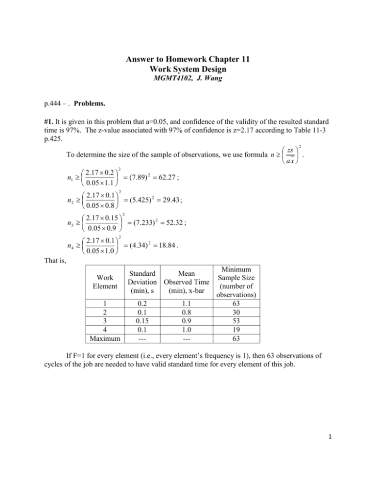
Answer to Homework Chapter 11
Work System Design
MGMT4102, J. Wang
p.444 – . Problems.
#1. It is given in this problem that a=0.05, and confidence of the validity of the resulted standard
time is 97%. The z-value associated with 97% of confidence is z=2.17 according to Table 11-3
p.425.
2
 zs 
To determine the size of the sample of observations, we use formula n    .
 ax 
 2.17  0.2 
2
n1  
  (7.89)  62.27 ;
 0.05  1.1 
2
 2.17  0.1 
2
n2  
  (5.425)  29.43 ;
0
.
05

0
.
8


2
 2.17  0.15 
2
n3  
  (7.233)  52.32 ;
 0.05  0.9 
2
 2.17  0.1 
2
n4  
  (4.34)  18.84 .
 0.05  1.0 
2
That is,
Work
Element
1
2
3
4
Maximum
Standard
Mean
Deviation Observed Time
(min), s
(min), x-bar
0.2
0.1
0.15
0.1
---
1.1
0.8
0.9
1.0
---
Minimum
Sample Size
(number of
observations)
63
30
53
19
63
If F=1 for every element (i.e., every element’s frequency is 1), then 63 observations of
cycles of the job are needed to have valid standard time for every element of this job.
1
#2. If confidence is set at 99%, then z=2.58.
 2.58  0.2 
2
n1  
  (9.38)  88.00 ;
 0.05  1.1 
2
 2.58  0.1 
2
n2  
  (6.45)  41.60 ;
0
.
05

0
.
8


2
 2.58  0.15 
2
n3  
  (8.60)  73.95 ;
 0.05  0.9 
2
 2.58  0.1 
2
n4  
  (5.16)  26.63 .
 0.05  1.0 
2
That is,
Work
Element
1
2
3
4
Maximum
Standard
Mean
Deviation Observed Time
(min), s
(min), x-bar
0.2
0.1
0.15
0.1
---
1.1
0.8
0.9
1.0
---
Minimum
Sample Size
(number of
observations)
88
42
74
27
88
If F=1 for every element (i.e., every element’s frequency is 1), then 88 observations of
cycles of the job are needed to have valid standard time for every element of this job.
2
#15. In this problem, the following are given or can be immediately derived:
Performance rating factors PRF;
Frequency of occurrence of an element F;
Personal time, Fatigue, and unavoidable Delay PFD=0.15;
1
1

 1.176 .
Allowance factor AF =
1  PFD 1  0.15
Mean observed time, MOT, for an element is the average of the given observed times for
the 15 observed cycles. The results are put in the second column of the table below.
In the table below,
“Mean observed time, MOT (min)” is calculated from the observed data of 15 cycles
given in the problem;
“PRF” and “F” are given,
“Normal time, NT (min)” is calculated by NT=(MOT)(PRF)(F);
“AF”=1.176 for the job therefore for every element, as calculate above;
“Standard time, ST (min)” is calculated by ST=NT*AF.
Element
1
2
3
4
5
Total
Mean
observed
time, MOT
(min)
0.582
1.515
0.759
0.319
2.1
PRF
F
0.95
0.9
1.0
1.1
0.9
1
0.25
1
1
0.2
Normal
time,
NT
(min)
0.5529
0.3409
0.759
0.3509
0.378
AF
1.176
1.176
1.176
1.176
1.176
Standard
time, ST
(min)
0.6502
0.4009
0.8926
0.4127
0.4445
2.8009
The standard time for the job is 2.8009 minutes per job .
(a) MOT for each element is shown in the table above.
(b) NT is shown in the table above.
(c) ST is shown in the table above.
(d) In an hour, a worker can complete: (60 min / 2.8009 min) = 21.42 units of the job.
(e) If worker performs 110% of the standard, he can complete (21.42*110%)=23.56 units.
3
#16. Given: percent error allowed e=0.05; confidence of the results = 0.97 (z=2.17), and
observed data of initial 20 observations.
2
z
To determine the size of the sample of observations, we use formula n    p (1  p) .
e
2
 2.17 
Since in this problem, z=2.17 and e=0.05, n  
 p (1  p )  1883.56 p (1  p ). Sample
 0.05 
proportions p are calculated from the initial trial observations as in the table below. The table
also shows the calculation of minimum size of observation samples for each activity.
(a) Answers are in the right column:
Number of Percent of
Activity
times
time
#
observed
observed, p
1
4
0.1
2
6
0.15
3
5
0.125
4
5
0.125
5
8
0.2
6
2
0.05
7
6
0.15
8
4
0.1
Total
40
1.0
Sample size = 1883.56 p(1-p)
1883.56*0.1*0.9 = 169.5 = 170
1883.56*0.15*0.85 = 240.2 = 241
1883.56*0.125*0.875 = 206.0 = 206
1883.56*0.125*0.875 = 206.0= 206
1883.56*0.2*0.8 = 301.4 = 302
1883.56*0.05*0.95 = 89.5 = 90
1883.56*0.15*0.85 = 240.2= 241
1883.56*0.1*0.9 = 169.5 = 170
Maximum = 302
After additional observations are taken, the observed occurrences, including the initial 40,
are summarized as:
Activity
#
Activity content
Number of
times observed
Proportion
1
2
3
4
5
6
7
8
Total
Grading
Administrative paperwork
Preparing for class
Teaching class
Meeting with student
On the phone
Working on research
Unavailable
-
30
50
30
30
66
17
45
34
302
0.0993
0.1656
0.0993
0.0993
0.2185
0.0563
0.1490
0.1126
0.9999
Hours
allocated in
54 hours
5.36
8.94
5.36
5.36
11.8
3.04
8.05
6.08
53.99
(b) Proportion of time on teaching class is 0.0993=9.93%.
(c) Proportion of time on research is 0.149=14.9%.
(d) See the column on the very right in the above table.
4
#17. Given: percent error allowed e=0.05; confidence of the results = 0.95, and observed data of
initial 20 observations.
The z-value for confidence=0.95 is z=1.96 according to Table 11-3 p.425 in textbook.
2
z
To determine the size of the sample of observations, we use formula n    p (1  p) .
e
2
 1.96 
Since in this problem, z=1.96 and e=0.05, n  
 p(1  p)  1536.64 p(1  p). Sample
 0.05 
proportions p are calculated from the initial trial observations as in the table below. The table
also shows the calculation of minimum size of observation samples for each activity.
Activity
With patient
Reviewing
test results
On phone
Idle
Away on
emergency
Not available
Total
Number of
times
observed
6
3
Percent of
time
Minimum sample size = 1536.64 p(1-p)
observed, p
0.3
1536.64*0.3*0.7 = 322.7 = 323
1536.64*0.15*0.85 = 195.9 = 196
0.15
2
1
0.1
0.05
4
0.2
4
20
0.2
1.0
1536.64*0.1*0.9 = 138.3 = 139
1536.64*0.05*0.95 = 73.0= 73
1536.64*0.2*0.8 = 245.9 = 246
1536.64*0.2*0.8 = 245.9 = 246
Maximum = 323
(a) Minimum sample size for activity “away on emergency” is 246.
(b) Minimum sample size for activity “reviewing test results” is 196.
(c) Minimum number of observations = maximum of sample sizes of activities = 323. (In order
to figure out the minimum number of observations, you need to compare the minimum sample
sizes in the right column of the above table and pick the maximum of them.)
5
#18.
T1=60 hours; Learning curve rate = L = 90%.
Formula TX = T1 * Ln is used to calculate the time used for the X-th time to do it, where
the value of Ln=LCCx can be found in Table 11-9 p.437 in the textbook. The value of Ln=LCCx
is at the intersection of row X (number of units) and column “90% - unit time”.
(a) For X=15, Ln=LCC15=0.663 from Table 11-9.
So, time needed for 15th installation is:
T15 = 60 * Ln = 60 * 0.663 = 39.78 (hours).
(b) For X=20, Ln=LCC20=0.634 from Table 11-9.
So, time needed for 20th installation is:
T20 = 60 * Ln = 60 * 0.634 = 38.04(hours)
(c) For X=20, Lntotal = cumulative LCCx = LCC1 + LCC2 + … + LCC20 = 14.608 from Table 11-9
at intersection of row 20 and column “90%-total time”.
So, total time needed for completing all 20 installations is:
Ttotal = 60 * Lntotal = 60 * 14.608 = 876.48 (hours)
(d) Total labor cost = ($32/hour)(876.48 hours) = $28,047.36.
#19.
T1=40 minutes; Learning curve rate = L = 80%.
Total time needed for Alexis to complete the 6-problem assignment is:
Ttotal = 40 * Lntotal = 40 * 4.299 = 171.96 (minutes) =2 hours and 51.96 minutes
where Lntotal = cumulative LCC6 = 4.299 is found in Table 11-9 p.437 at intersection of row 6
and column “80%-total time”.
6