eAppendix of ” A sensitivity analysis formula for unmeasured confounding for the
attributable fraction.”
To derive Result 1, we require the following assumptions. First, we assume that the
potential outcome Ya for an individual does not depend on the exposure status of other individuals.
This assumption is sometimes referred to as the stable unit treatment value assumption1 or as a
no-interference assumption.2 Second, we require the consistency assumption YA = Y; i.e., the value
of Y that would have been observed if A had been set to its actual value is equal to the actually
observed value of Y. Therefore, the only potential outcome for an individual that we observe is the
potential outcome YA; i.e., the value of Y that would have been observed if A was set to its actual
value. Third and finally, we suppose that the effect of A on Y is unconfounded given both X and U;
in counterfactual notation, Ya is independent of A conditional on X and U, where U is an
unmeasured confounder or a set of unmeasured confounders.
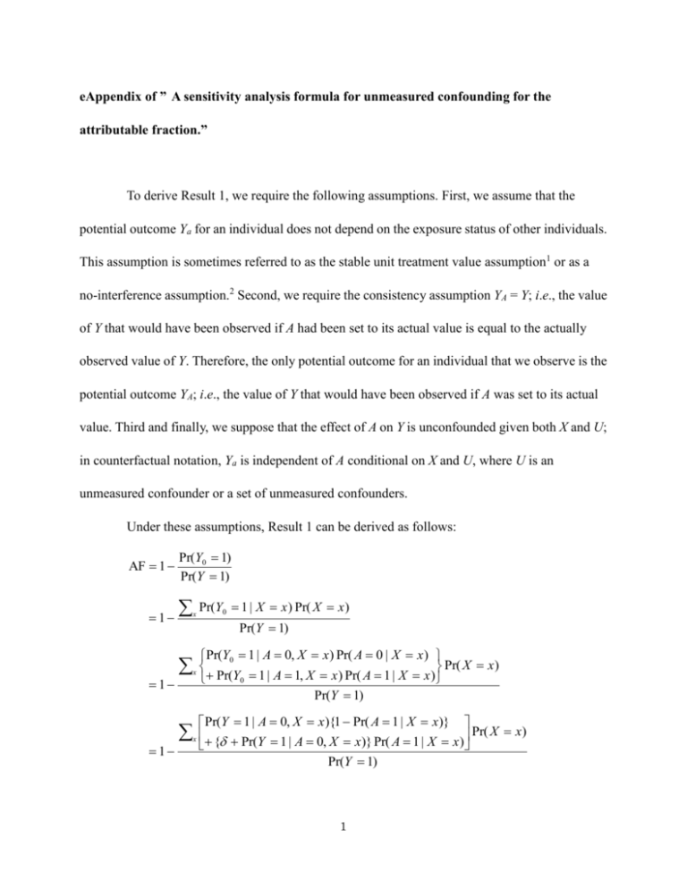
Under these assumptions, Result 1 can be derived as follows:
AF  1 
 1
1
1
Pr(Y0  1)
Pr(Y  1)

x
Pr(Y0  1 | X  x ) Pr( X  x )
Pr(Y  1)
Pr(Y0  1 | A  0, X  x ) Pr( A  0 | X  x ) 
 Pr( X  x )
x
 Pr(Y0  1 | A  1, X  x ) Pr( A  1 | X  x ) 
Pr(Y  1)

 Pr(Y  1 | A  0, X  x ){1  Pr( A  1 | X  x )} 
 Pr( X  x )
x
 {  Pr(Y  1 | A  0, X  x )} Pr( A  1 | X  x )
Pr(Y  1)

1
1

x
 AF O 
Pr(Y  1 | A  0, X  x ) Pr( X  x )
Pr(Y  1)

  Pr( X  x | A  1) Pr( A  1)
x
Pr(Y  1)
Pr( A  1)
.
Pr(Y  1)
eAppendix references
1.
Rubin DB. Formal models of statistical inference for causal effects. J Stat Plan Infer.
1990;25:279–292.
2.
Cole SR, Hernán MA. Constructing inverse probability weights for marginal structural models.
Am J Epidemiol. 2008;168:656–664.
2