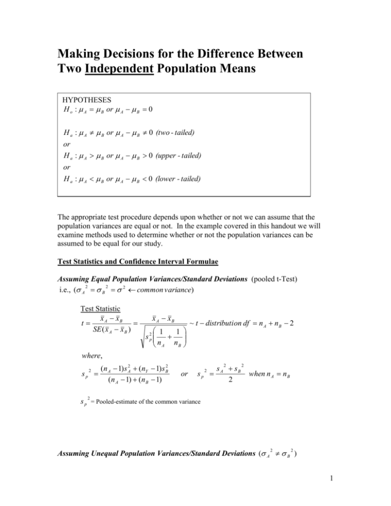
Making Decisions for the Difference Between
Two Independent Population Means
HYPOTHESES
H o :  A   B or  A   B  0
H a :  A   B or  A   B  0 (two - tailed)
or
H a :  A   B or  A   B  0 (upper - tailed)
or
H a :  A   B or  A   B  0 (lower - tailed)
The appropriate test procedure depends upon whether or not we can assume that the
population variances are equal or not. In the example covered in this handout we will
examine methods used to determine whether or not the population variances can be
assumed to be equal for our study.
Test Statistics and Confidence Interval Formulae
Assuming Equal Population Variances/Standard Deviations (pooled t-Test)
2
2
i.e., ( A   B   2  common variance)
Test Statistic
x A  xB
t

SE ( x A  x B )
x A  xB
 1
1
s 2p 

 n A nB



~ t  distributi on df  n A  n B  2
where,
sp
2
(n A  1) s A2  (nY  1) s B2

(n A  1)  (n B  1)
s  sB
 A
2
2
or
sp
2
2
when n A  n B
2
s p = Pooled-estimate of the common variance
Assuming Unequal Population Variances/Standard Deviations ( A   B )
2
2
1
Test Statistic
x A  xB
t

SE ( x A  x B )
x A  xB
2
2
sA
s
 B
nA
nB
~ t-distribution
df = min( n A  1, nB  1 )
This is the conservative approach. As an alternative we
could use Welch’s df formula, but for Welch’s we will
let the computer do the dirty work!
Confidence Interval for the Difference Between the Pop. Means
For either case a CI for ( A   B ) is given by the following
(estimate) + (t-table value)(standard error of estimate)
( x A  xB )  t  SE( x A  xB )  (margin of error is computing using the appropriate standard error
and df based upon the equality of pop. variances assumption)
EXAMPLE 1: NORMAL HUMAN BODY TEMPERATURE:
FEMALES vs. MALES
Data File: Bodytemp.JMP
Background: The data for this example comes from a study of body temperature and pulse rate
for adults.
Variables: Gender: gender of the individual
Temperature: body temperature (degrees Farenheit)
Heart.rate: heart or pulse rate (beat per minute)
Goal: To be able to complete (and interpret the output from) a two-sample t-test in JMP.
Question of Do men and women have the same normal body temperature? Putting this statement
Interest: into a statement involving parameters that can be tested:
HO: F = M
HA: F ≠ M
or
 F  mean body temperature for females.
 M  mean body temperature for males.
HO: F - M= 0
HA: F - M ≠ 0
Intuitive Decision
In order to determine whether or not the null or alternative hypothesis is true, you could
review the summary statistics for the variable you are interested in testing across the two
groups. Remember, these summary statistics and/or graphs are for the observations you
sampled, and to make decisions about all observations of interest, we must apply some
inferential technique (i.e. hypothesis tests or confidence intervals)
2
One of the best graphical displays for this situation is the side-by-side boxplots. To get
side-by-side boxplots, select Analyze > Fit Y by X. Place Gender in the X box and
Temperature in the Y box. Place the mean diamonds on the boxplots and jitter the
points. The more separation there is in the mean diamonds, the more likely we are to
reject the null hypothesis (i.e data tends to support the alternative hypothesis).
Summary Statistics
x F  98.39
x M  98.10
s F  .743
s M  .699
n F  65
n M  65
Assumptions
1. The two groups must be independent of each other.
2. The observation from each group should be normally distributed.
3. Decide whether or not we wish to assume the population variances are equal.
Assessing Normality of the Two Sampled Populations
To assess normality we select Normal Quantile Plot from the Oneway Analysis pulldown menu as shown below.
Normality appears to
be satisfied here.
3
Checking the Equality of the Population Variances
To test the equality of the population variances select Unequal Variances from the
Oneway Analysis pull-down menu.
The test is:
JMP gives four different tests for examining the equality of population variances. To use
the results of these tests simply examine the resulting p-values. If any/all are less than .10
or .05 then worry about the assumption of equal variances and use the unequal variance tTest instead of the pooled t-Test.
Here we can see that all of the p-values exceed the 0.05 (i.e. 5%). What does this mean?
What is your conclusion about the validity of the equality of the population variances
assumption?
4
Performing the Test
To perform the two-sample t-test for independent samples:
 assuming equal population variances select the Means/Anova/Pooled t option
from Oneway-Analysis pull-down menu.
 assuming unequal population variances select t-Test from the Oneway-Analysis
pull-down menu.
Because we have no evidence
against the equality of the
population variances
assumption we will use a
pooled t-Test to compare the
population means.
Several new boxes of output will appear below the graph once the appropriate option has
been selected, some of which we will not concern ourselves with. The relevant box for us
will be labeled t Test as shown below for the mean body temperature comparison.
Because we have concluded
that the equality of variance
assumption is reasonable for
these data we can refer to the
output for the t-Test assuming
equal variances.

Summary Statistics
What is the test statistic for this test?
x F  98.39
x M  98.10
s F  .743
s M  .699
n F  65
n M  65
t
x A  xB

SE ( x A  x B )
x A  xB
 1
1 

s 

n
n
A
B 

~ t  distributi on df  n A  n B  2
2
p
where,
sp 
2
(n A  1) s A2  (nY  1) s B2
(n A  1)  (n B  1)
s A  sB
2
2
or
sp 
2
5
2
when n A  n B

What is the p-value?

What is your decision for the test?

Write a conclusion for your findings.
Construct and Interpret a 95% CI for the Difference in the
Mean Body Temperatures ( F   M )
Summary Statistics
For body temperature and gender example we have:
x F  98.39
x M  98.10
s F  .743
s M  .699
n F  65
n M  65
t
x A  xB

SE ( x A  x B )
x A  xB
 1
1 
s 


n
n
B 
 A
~ t  distributi on df  n A  n B  2
2
p
where,
sp 
2
Interpretation of the CI for ( F   M )
(n A  1) s A2  (nY  1) s B2
(n A  1)  (n B  1)
s A  sB
2
2
or
sp 
2
( A   B )
( x A  xB )  t  SE( x A  xB )
CI for
6
2
when n A  n B
Nonparametric Alternative to the t-Test (not on an exam)
If we find that the populations we are sampling from are not normally distributed or if our
samples are too small to reasonably assess normality we could use a nonparametric test
instead. Nonparametric tests typically use the ranks of the observations rather than the
observed values themselves to compare the “size” of the values from the two populations
of interest. All the observations from both samples are ranked from smallest to largest
with the smallest observation receiving a rank of 1. The general idea of the test is to
compare the ranks of assigned to the observations from each population. If one
population generally has larger values than the other, the observations sampled from that
population should have significantly higher ranks than the observations sampled from the
population with smaller values. If the discrepancy in the ranks is extreme enough we will
reject the null that says the population distributions are the same in terms of “typical”
value in favor of the alternative which says that one population has larger values than the
other.
To perform a nonparametric test of this hypotheses in JMP select Nonparametric >
Wilcoxon from the Oneway Analysis pull-down menu. The normal approximation pvalue is virtually identical to the normal approximation to the Mann -Whitney test. Here
the conclusion is the same as the parametric test, namely males and females have
significantly different body temps.
7
Example 2: Gender Comparisons of Drinks Per Episode
for WSU Students
Is there evidence to suggest that the average number of drinks per episode for male
drinkers is greater than that for female drinkers? Using the WSU student survey data in
the file STAT 110 Survey we will examine this question.
H o : F  M
H A : F  M
 F  mean number of drinks per episode for WSU females
 M  mean number of drinks per episode for WSU males
Analysis in JMP
Using Analyze > Fit Y by X with Y = Howmuch, which is the number of drinks per
episode, and X = Gender we obtain the following. Select Oneway Analysis... > Normal
Quantile Plot to assess normality of the response for both groups.
Both distributions
are skewed right,
however our
sample sizes here
are quite large so
normality is less
critical.
Can we assume the population variances are equal? Select Oneway Analysis >
UnEqual Variances to check this assumption. The results are shown on the following
page.
8
What do we conclude?
Using the appropriate t-Test given the variance test results we select Oneway Analysis...
> t Test.
Conclusion:
Results
9
Additional Notes:
10