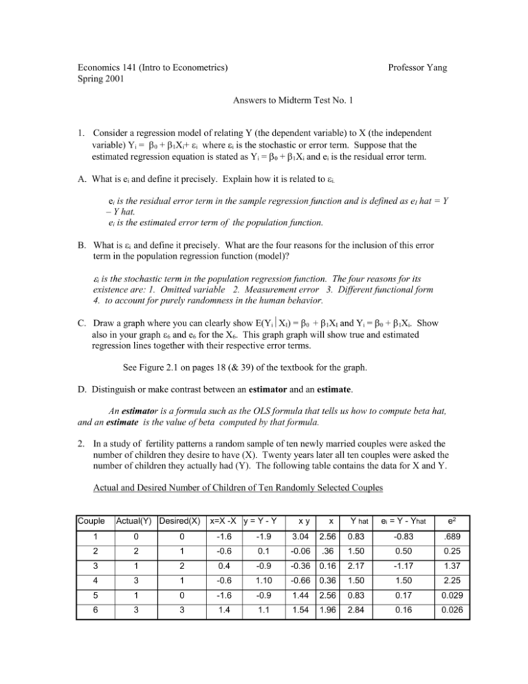
Economics 141 (Intro to Econometrics)
Spring 2001
Professor Yang
Answers to Midterm Test No. 1
1. Consider a regression model of relating Y (the dependent variable) to X (the independent
variable) Yi =  0 + 1Xi+ i where i is the stochastic or error term. Suppose that the
estimated regression equation is stated as Yi =  0 + 1Xi and ei is the residual error term.
A. What is ei and define it precisely. Explain how it is related to i.
ei is the residual error term in the sample regression function and is defined as eI hat = Y
– Y hat.
ei is the estimated error term of the population function.
B. What is i and define it precisely. What are the four reasons for the inclusion of this error
term in the population regression function (model)?
i is the stochastic term in the population regression function. The four reasons for its
existence are: 1. Omitted variable 2. Measurement error 3. Different functional form
4. to account for purely randomness in the human behavior.
C. Draw a graph where you can clearly show E(YiXI) =  + XI and Yi = 0 + 1Xi. Show
also in your graph  and e6 for the X6. This graph graph will show true and estimated
regression lines together with their respective error terms.
See Figure 2.1 on pages 18 (& 39) of the textbook for the graph.
D. Distinguish or make contrast between an estimator and an estimate.
An estimator is a formula such as the OLS formula that tells us how to compute beta hat,
and an estimate is the value of beta computed by that formula.
2. In a study of fertility patterns a random sample of ten newly married couples were asked the
number of children they desire to have (X). Twenty years later all ten couples were asked the
number of children they actually had (Y). The following table contains the data for X and Y.
Actual and Desired Number of Children of Ten Randomly Selected Couples
Couple
Actual(Y) Desired(X)
x=X -X y = Y - Y
xy
x
Y hat
ei = Y - Yhat
e2
1
0
0
-1.6
-1.9
3.04
2.56
0.83
-0.83
.689
2
2
1
-0.6
0.1
-0.06
.36
1.50
0.50
0.25
3
1
2
0.4
-0.9
-0.36
0.16
2.17
-1.17
1.37
4
3
1
-0.6
1.10
-0.66
0.36
1.50
1.50
2.25
5
1
0
-1.6
-0.9
1.44
2.56
0.83
0.17
0.029
6
3
3
1.4
1.1
1.54
1.96
2.84
0.16
0.026
7
4
4
2.4
2.1
5.04
5.76
3.51
0.49
0.24
8
2
2
0.4
0.1
0.04
0.16
2.17
-0.17
0.029
9
1
2
0.4
-0.9
-0.36
0.16
2.17
-1.17
1.37
10
2
1
-0.6
0.1
-0.06
0.36
1.5
0.5
0.25
SUM
19
16
0
0
9.6
14.4
19.02
-0.02
6.50
A. Calculate the covariance and correlation coefficient between Y and X.
Use Cov Y,X =  x y / N-1 and CorrY,X = CovY,X / X Y. Also X bar= 1.6 and Y bar= 1.9
Cov Y,X =
9.6 /9 = 1.0067
Corr Y,X =
1.067 / 1.26 * 1.20 = 1.067 / 1.512 = 0.706
Var (X) =  x2 / N-1 = 14.4 / 9 = 1.6
Var(Y) = y2 /N-1 = 12.9 /9 = 1.433
X = sq root of 1.6 =1.26
Y = sq. root of 1.433 =1.20
B. For a linear regression model of Y =  + XI + i, estimator for coefficient for
 =  xi yi /  xi2 where xi = Xi - X and yi = Yi – Y. Given the estimate of ,  can be
found by  = Y -  X. Using information for X and Y and X in the above table, calculate.
and . 1 =  xy /  x2 = 9.6 / 14.4 = 0.667
0 = Y bar – beta hat X bar = 1.9 – 0.67 * 1.6 = 0.83
2) Interpret the economic meaning of the estimated coefficients for  and .
With one unit increase in the desired number of children of newly married couples, 0.67
additional children increases on the average.
No particular economic meaning for beta zero (intercept term).
3) Calculate the variance of the regression. To do this, you need to calculate first the estimated
residuals e = Yi – Y and then calculate the sum of the squared residuals in the table.
Variance of the regression =  e2 / N-k-1 = 6.50 / 8 = 0.8125
3. A. State the underlying assumptions for the classical linear regression model stated below:
Yi =  + 1 Xi + 2 Zi + i
1.
2.
3.
4.
5.
6.
7.
Correctly specified, linearity in the coefficient, and additive error term.
E( ) = 0
Explanatory variables are not correlated with the error term, Cov(X,  ) = 0
No serial correlation.
Homoschedasticity.
No multicollinearity.
Normality of the error term.
B. Graphically illustrate the following assumptions: E(i) = 0, Var() = 2 , Var(I)  2.
See the hand-outs from Gujarati’s textbook.
C. One of the implication of the normality assumption of  in the classical linear
regression model is that the s are also normally distributed. This means that there are different
values of s, which is assumed to follow the normal distribution. But when one obtains a
particular  from a set of data, it is a fixed number. How do you reconcile the two? Is  a fixed
number or does it follow a normal distribution? Justify your answer.
 hat obtained from one sample is a fixed number, while the normal distribution of  hat is to
be obtained from repeated random samplings.
4. Consider the following model
Yt =  +  Xt + 2 Xt + t
Where Yt = actual rate of inflation (%) at time t, X2t =unemployment rate (%) at time t, and X3t =
expected inflation rate (%) at time t. This model is known as the expectations-augmented Phillips
curve.
As a test of this model, we obtained the data and the OLS method gave the following results.
Yt = 7.1933 – 1.3925 X2t + 1.4700 X3t
R2 = 0.50
A. Hypothesize the expected signs of the coefficients  and .
From macroeconomic theory of the Phillips curve notion of aggregate supply, we
hypothesize that the sign of the coefficient for the unemployment rate is negative,
indicating a trade-off between the rate of inflation and unemployment rate.
From again expectation-augmented Phillips curve, the hypothesized relationship between
the inflation rate and expected inflation rate is positive.
B. Carefully state the meaning of the coefficients –1.3925 and 1.4700 in the equation in terms
of the impact of X2t and X3t on Y.
As unemployment rate increases by one percent, its expected impact on the rate of inflation
is to lower the inflation rate by 1.3925 % on the average, when holding other determinant,
namely the expected inflation rate constant.
C. What is R2 bar and what does R2 bar= 0.50 means? Why does one prefer to use R2 bar
rather than R2?
R2 bar is a measure of goodness of fit and is equal to ESS/TSS. R bar square is a
measure of goodness of fit adjusted for the degrees of freedom.
R2 bar of 0.50 means that 50% of the variation in the dependent variable Y from its mean
is explained by the estimated regression. One prefers R bar square to R squares, for the former
adjusts for the degrees of freedom.
D. Suppose that you were told that the true value of  is –1.20. Does this show that the
estimate is biased? Why or why not?
No. The estimate of –1.3925 is only one estimate of beta from one sample. Estimation
of s from repeated random samplings will yield a normal distribution of s and the mean of the 
hat can be equal to true value of –1.20.
5. Assuming that all seven classical assumptions, the OLS estimators  and  can have
several desirable properties. List those properties and explain concisely what each means.
1. They are unbiased. This means that the OLS estimates of the coefficients are
centered around the true population values of the parameters being estimated.
2. They are minimum variance. This means that no other unbiased estimator has a
lower variance for each s than OLS.
3. They are consistent. This means that as the sample size approaches infinity, the
estimates converge on the true population parameters.
4. They are normally distributed.