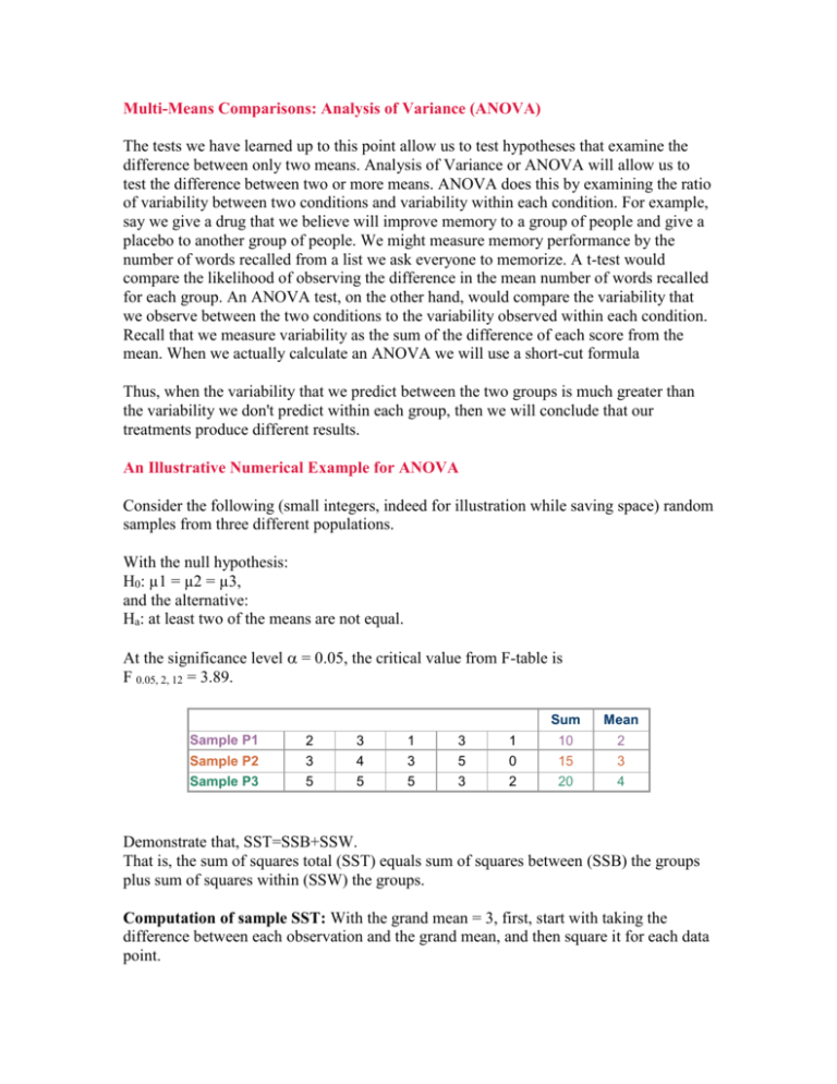
Multi-Means Comparisons: Analysis of Variance (ANOVA)
The tests we have learned up to this point allow us to test hypotheses that examine the
difference between only two means. Analysis of Variance or ANOVA will allow us to
test the difference between two or more means. ANOVA does this by examining the ratio
of variability between two conditions and variability within each condition. For example,
say we give a drug that we believe will improve memory to a group of people and give a
placebo to another group of people. We might measure memory performance by the
number of words recalled from a list we ask everyone to memorize. A t-test would
compare the likelihood of observing the difference in the mean number of words recalled
for each group. An ANOVA test, on the other hand, would compare the variability that
we observe between the two conditions to the variability observed within each condition.
Recall that we measure variability as the sum of the difference of each score from the
mean. When we actually calculate an ANOVA we will use a short-cut formula
Thus, when the variability that we predict between the two groups is much greater than
the variability we don't predict within each group, then we will conclude that our
treatments produce different results.
An Illustrative Numerical Example for ANOVA
Consider the following (small integers, indeed for illustration while saving space) random
samples from three different populations.
With the null hypothesis:
H0: µ1 = µ2 = µ3,
and the alternative:
Ha: at least two of the means are not equal.
At the significance level = 0.05, the critical value from F-table is
F 0.05, 2, 12 = 3.89.
Sum
Mean
Sample P1
2
3
1
3
1
10
2
Sample P2
3
4
3
5
0
15
3
Sample P3
5
5
5
3
2
20
4
Demonstrate that, SST=SSB+SSW.
That is, the sum of squares total (SST) equals sum of squares between (SSB) the groups
plus sum of squares within (SSW) the groups.
Computation of sample SST: With the grand mean = 3, first, start with taking the
difference between each observation and the grand mean, and then square it for each data
point.
Sum
Sample P1
1
0
4
0
4
9
Sample P2
0
1
0
4
9
14
Sample P3
4
4
4
0
1
13
Therefore SST = 36 with d.f = (n-1) = 15-1 = 14
Computation of sample SSB:
Second, let all the data in each sample have the same value as the mean in that sample.
This removes any variation WITHIN. Compute SS differences from the grand mean.
Sum
Sample P1
1
1
1
1
1
5
Sample P2
0
0
0
0
0
0
Sample P3
1
1
1
1
1
5
Therefore SSB = 10, with d.f = (m-1)= 3-1 = 2 for m=3 groups.
Computation of sample SSW:
Third, compute the SS difference within each sample using their own sample means. This
provides SS deviation WITHIN all samples.
Sample P1
0
1
1
1
1
Sum
4
Sample P2
0
1
0
4
9
14
Sample P3
1
1
1
1
4
8
SSW = 26 with d.f = 3(5-1) = 12. That is, 3 groups times (5 observations in each -1)
Results are: SST = SSB + SSW, and d.fSST = d.fSSB + d.fSSW, as expected.
Now, construct the ANOVA table for this numerical example by plugging the results of
your computation in the ANOVA Table. Note that, the Mean Squares are the Sum of
squares divided by their Degrees of Freedom. F-statistics is the ratio of the two Mean
Squares.
The ANOVA Table
Sources of Variation Sum of Squares Degrees of Freedom Mean Squares F-Statistic
Between Samples
10
2
5
2.30
Within Samples
26
12
2.17
Total
36
14
Conclusion: There is not enough evidence to reject the null hypothesis H0.
The Logic behind ANOVA: First, let us try to explain the logic and then illustrate it
with a simple example. In performing the ANOVA test, we are trying to determine if a
certain number of population means are equal. To do that, we measure the difference of
the sample means and compare that to the variability within the sample observations.
That is why the test statistic is the ratio of the between-sample variation (MSB) and the
within-sample variation (MSW). If this ratio is close to 1, there is evidence that the
population means are equal.
Here is a good application for you: Many people believe that men get paid more in the
business world, in a specific profession at specific level, than women, simply because
they are male. To justify or reject such a claim, you could look at the variation within
each group (one group being women's salaries and the other group being men's salaries)
and compare that to the variation between the means of randomly selected samples of
each population. If the variation in the women's salaries is much larger than the variation
between the men's and women's mean salaries, one could say that because the variation is
so large within the women's group that this may not be a gender-related problem.
Now, getting back to our numerical example of the drug treatment to improve memory
vs. the placebo, we notice that: given the test conclusion and the ANOVA test's
conditions, we may conclude that these three populations are in fact the same population.
Therefore, the ANOVA technique could be used as a measuring tool and statistical
routine for quality control as described below using our numerical example.
Construction of the Control Chart for the Sample Means: Under the null hypothesis,
the ANOVA concludes that µ1 = µ2 = µ3; that is, we have a "hypothetical parent
population." The question is, what is its variance? The estimated variance (i.e., the total
mean squares) is 36 / 14 = 2.57. Thus, estimated standard deviation is = 1.60 and
estimated standard deviation for the means is 1.6 / 5½  0.71. Under the conditions of
ANOVA, we can construct a control chart with the warning limits = 3 ± 2(0.71); the
action limits = 3 ± 3(0.71). The following figure depicts the control chart.
Conditions for Using ANOVA Test: The following conditions must be tested prior to
using ANOVA test otherwise the results are not valid: Randomness of the samples,
Normality of populations, and Equality of Variances for all populations.
You May Ask Why Not Using Pair-wise T-test Instead ANOVA? Here are two
reasons: Performing pair-wise t-test for K populations, you will need to perform, K(K1)/2 pair-wise t-test. Now suppose the significance level for each test is set at 5% level,
then the overall significance level would be approximately equal to 0.05K(K-1)/2. For
example, for K = 5 populations, you have to performing 10 pair-wise t-tests, moreover,
the overall significance level is equal to 50%, which is too high type-I error for any
statistical decision making.
You might like to use ANOVA: Testing Equality of Means for your computations, and
then to interpret the results in managerial (not technical) terms.