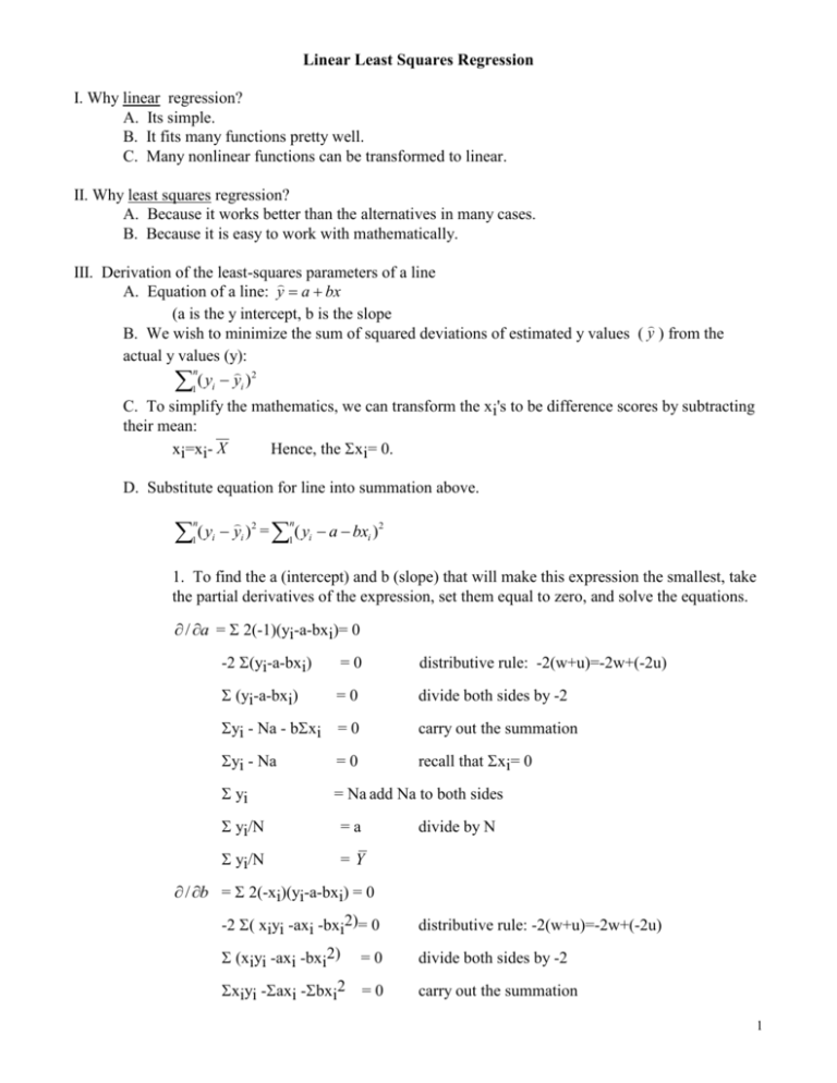
Linear Least Squares Regression
I. Why linear regression?
A. Its simple.
B. It fits many functions pretty well.
C. Many nonlinear functions can be transformed to linear.
II. Why least squares regression?
A. Because it works better than the alternatives in many cases.
B. Because it is easy to work with mathematically.
III. Derivation of the least-squares parameters of a line

A. Equation of a line: y  a  bx
(a is the y intercept, b is the slope

B. We wish to minimize the sum of squared deviations of estimated y values ( y ) from the
actual y values (y):
n

1 ( yi  yi )2
C. To simplify the mathematics, we can transform the xi's to be difference scores by subtracting
their mean:
xi=xi- X
Hence, the xi= 0.
D. Substitute equation for line into summation above.

 ( y  y ) =  ( y  a  bx )
n
1
i
2
i
n
1
i
2
i
1. To find the a (intercept) and b (slope) that will make this expression the smallest, take
the partial derivatives of the expression, set them equal to zero, and solve the equations.
 / a =  2(-1)(yi-a-bxi)= 0
-2 (yi-a-bxi)
=0
distributive rule: -2(w+u)=-2w+(-2u)
 (yi-a-bxi)
=0
divide both sides by -2
yi - Na - bxi
=0
carry out the summation
yi - Na
=0
recall that xi= 0
 yi
= Na add Na to both sides
 yi/N
=a
 yi/N
=Y
divide by N
 / b =  2(-xi)(yi-a-bxi) = 0
-2 ( xiyi -axi -bxi2)= 0
distributive rule: -2(w+u)=-2w+(-2u)
 (xiyi -axi -bxi2)
=0
divide both sides by -2
xiyi -axi -bxi2
=0
carry out the summation
1
xiyi -axi -bxi2
=0
distributive rule again
 xiyi - b xi2
=0
recall that xi= 0
 xiyi
= b xi2
 xiyi/ xi2
= b
add bxi2 to both sides
divide by xi2
IV. Goodness of fit of regression model
A. Decomposition of variation
Total SS = SS regression + SS residual
Total variation around mean of Y= variation “explained” by line + unexplained
variation around line.
n
n
n

1 ( yi  Y )2 = 1 ( yˆi  Y )2 + 1( yi  yi )2
B. Proportion of variance explained by line

( yi  Y ) 2
Explained variation

1.
=
Total variation
 ( yi  Y )2
= ryy
2
C. Estimate of variance 2

( yi  yi ) 2

2
s=
N  k 1
where k=number of predictors (in linear regression=1). Note: 2 df are lost, 1 for
each parameter estimated (no variance with only 2 points)
D. F-ratio testing variance explained by line

( yi  Y ) 2 df reg
MS regression

=

MS residual
 ( yi  yi )2 df res
dfreg = k = # of predictors; dfres = N-k-1
V. Testing parameters of regression model
A. Purpose
1. The estimated a and b are sample estimates of the true population parameters. Want
to determine how close the sample estimates are to the true population parameters.
2. Confidence intervals give a range of values within which the population parameters
will lie with a stated degree of certainty ().
3. Tests of significance ask whether for some given degree of certainty, the population
value of a parameter may be different from some given value (usually 0).
B. Standard Assumptions
1. Given a regression model: yi=a + bxi + ei
2. yi are independently and identically distributed with variance 2.
3. ei are independently and identically distributed with mean 0 and variance 2.
4. xi are fixed (not random variables).
2
C. Statistics for b
1. Derivation of variance of b
see above
b = xiyi/xi2
= (xi/xi2)yi
distributive rule
= wiyi
rewrite equation; let wi=xi/xi2
so, b is a linear combination of random variables
var(b) = wi2var(yi)
variance of linear combination of random variables
2
2
= wi 
by assumption 2 above
2
2
replacing wi by its equivalent
= xi 
(xi2)2
simplifying by canceling one xi2
= 2
xi2
2. Standard error of b
sb =
var(b) =
s
x
2
i
3. T-test for b
b
t=
df=N-k-1
sb
4. Confidence interval for b
s
ß = b ± t/2
 xi 2
5. Note: large variation in x will yield smaller sb and larger t. With small variation in x,
estimates are unstable.
D. The constant is rarely of interest. When it is, similar tests can be performed. Note that the
constant is simply the regression coefficient for a predictor that does not vary in the data. The
variance of a = 2/n.
VI. Problems
A. Outliers
1. There may be observations for which the relation(s) between the criterion and the
predictor(s) are not summarized well by the regression equation.
B. Heteroscedasticity
1. The variance around the regression line may not be constant. Hence, the equation
predicts better in some ranges than in others.
C. Curvilinearity
1. The regression line may systematically underestimate in some ranges and overestimate
in others because the relation between the criterion and the predictor(s) is not linear.
D. Autocollinearity
1. The observations (and the residuals) may be correlated (frequently a problem with
time series data) yielding inaccurate parameter estimates that may appear to be more
precise than they really are.
3
E. Nonlinearity
1. The relation(s) between the predictor(s) and the criterion may be nonlinear. For
example:
a. y= a + bx +bx2 + e
b. y= a + bln(x) + e
2. Note that in some cases, relations that are theoretically nonlinear may be transformed
into linear relations.
a. Example - learning theory transformed to linear
ti = abxi
a > 0 [positive]
0<b<1 [fraction]
ti = time taken to perform task on ith occasion
xi = # of trials
b. Converted to linear
ln(ti) = ln(abxi)
taking natural log of both sides
= ln(a) + ln(bxi)
ln(w*u)=ln(w)+ln(u)
= ln(a) + xln(b)
ln(wu)=u*ln(w)
3. However, some relations cannot be transformed to linear (intractable nonlinearity).
VII. Detection of Problems
A. Think about the data
1. What relations between the variables might be expected?
2. What problems may occur?
B. Plot the data
1. Plot criterion by predictors and examine form and spread
C. Plot the residuals after performing the regression.
1. Plot residuals or standardized residuals by predicted values of the criterion.
D. Examine diagnostic statistics for the presence of outliers.
1. Large residuals
a. Some authors suggest the rule of thumb that any standardized residual > 2
requires inspection.
b. Some authors suggest examining studentized residuals because the residuals
may not be homoscedastic. The studentized residual is calculated by dividing
each residual by its estimated standard deviation. The estimated standard
deviation of a residual is defined as:
 1 ( x  X )2 
sei  s 1    i

 N
 xi 2 
where s=standard error of the estimate (see above).
The studentized residuals can then be tested against a t distribution with N-k-1
degrees of freedom. Note that in practice this is not an appropriate test because
the t tests are not independent. However, it is a way of locating unusually large
residuals.
4
2. Leverage
a. Some authors suggest examining the “leverage” of an observation, defined as
the quantity in brackets above:
 1 ( x  X )2 
hi =   i

 N
 xi 2 
A large leverage is an indication that the value of the predictor is far from the
mean of that predictor.
3. Cook’s D (Cook, 1977)
a. Leverage does not measure the influence of an observation on the criterion.
Cook’s D does:
 esi 2   hi 
Di  


 k  1 1  hi 
where esi2 = studentized residual for observation i; hi=leverage for observation i.
Approximate tests of the significance of D are available, but usually one
simply looks for D’s that are large relative to the others in the dataset.
4. Delete suspect observations
a. One should be able to delete points without substantial effect on parameters. If
one cannot, then either the number of observations is too small or the observation
in question is an outlier.
b. Some computer programs routinely report DFBETAi which is the regression
coefficient that would result were observation i to be deleted.
5