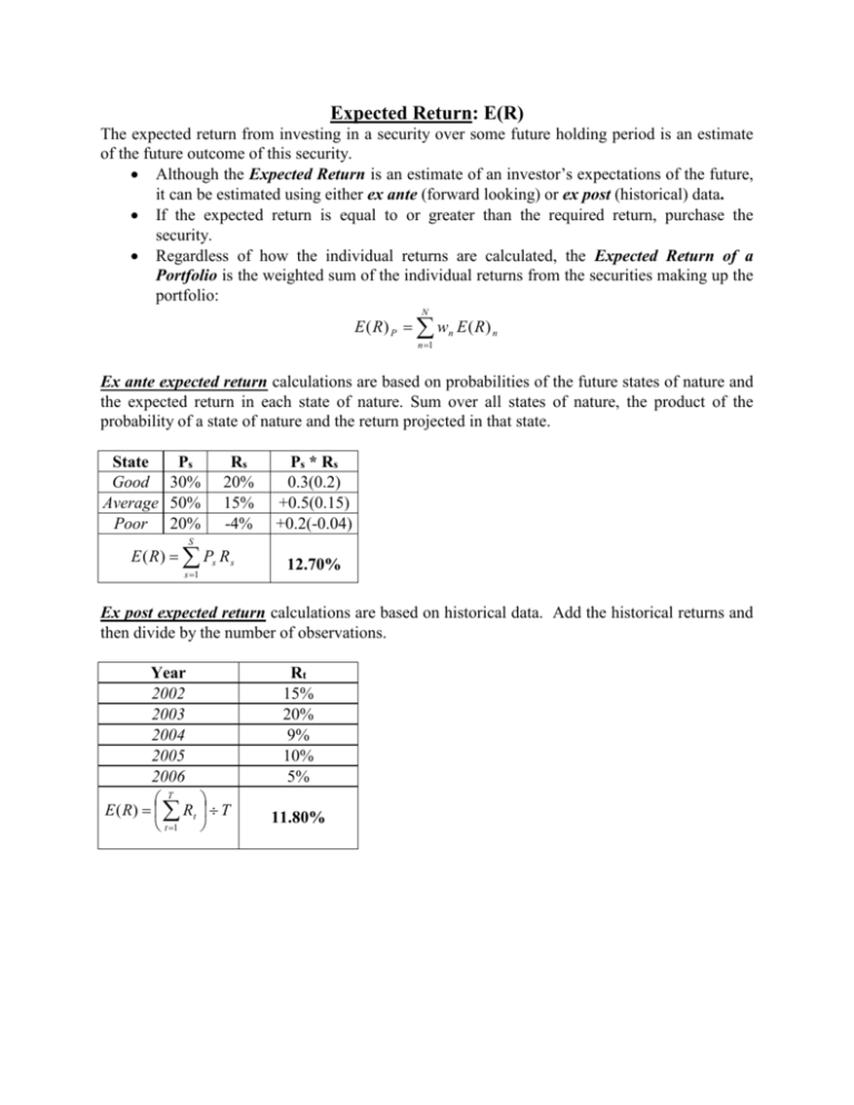
Expected Return: E(R)
The expected return from investing in a security over some future holding period is an estimate
of the future outcome of this security.
 Although the Expected Return is an estimate of an investor’s expectations of the future,
it can be estimated using either ex ante (forward looking) or ex post (historical) data.
 If the expected return is equal to or greater than the required return, purchase the
security.
 Regardless of how the individual returns are calculated, the Expected Return of a
Portfolio is the weighted sum of the individual returns from the securities making up the
portfolio:
N
E ( R ) P   wn E ( R ) n
n 1
Ex ante expected return calculations are based on probabilities of the future states of nature and
the expected return in each state of nature. Sum over all states of nature, the product of the
probability of a state of nature and the return projected in that state.
State
Ps
Good 30%
Average 50%
Poor 20%
Rs
20%
15%
-4%
Ps * Rs
0.3(0.2)
+0.5(0.15)
+0.2(-0.04)
S
E ( R )   Ps R s
s 1
12.70%
Ex post expected return calculations are based on historical data. Add the historical returns and
then divide by the number of observations.
Year
2002
2003
2004
2005
2006
 T

E ( R )    Rt   T
 t 1 
Rt
15%
20%
9%
10%
5%
11.80%
Variance (Standard Deviation): σ2 (σ)
Variance is a measure of the dispersion in outcomes around the expected value. It is used as an
indication of the risk inherent in the security. Standard deviation is the square root of variance.
Ex ante variance calculation:
1. The expected return is subtracted from the return within each state of nature; this
difference is then squared.
2. Each squared difference is multiplied by the probability of the state of nature.
3. These weighted squared terms are then summed together.
State
Ps
Good 30%
Average 50%
Poor 20%
Ps * Rs
(Rs – E(R))2 * Ps
0.3(0.2)
0.3(0.2-0.127)2
+0.5(0.15) +0.5(0.15-0.127)2
+0.2(-0.04) +0.2(-0.04-0.127)2
12.70%
0.0074
Mean
Variance
Rs
20%
15%
-4%
S
 2   [ R s  E ( R)] 2 Ps
8.63%
Standard
Deviation
  2
s 1
Ex post variance calculation:
1. The average return is subtracted from each single period return; this difference is then
squared.
2. The squared differences are summed.
3. This sum is divided by the number of periods (using population data) or the number of
periods minus 1 (using sample data).
Year
2002
2003
2004
2005
2006
Population
data
Sample
data
(Rt – E(R))2
(0.15-0.118)2
(0.2-0.118)2
(0.09-0.118)2
(0.1-0.118)2
(0.05-0.118)2
=Sum/4
0.0034
Sample
Variance
5.81%
Sample
Std Dev
T


 2   ( Rt  E ( R)) 2   (T )
 t 1

T


 2   ( Rt  E ( R)) 2   (T  1)
 t 1

Rt
15%
20%
9%
10%
5%
= Sum/5
11.80%
Mean
(Rt – E(R))2
(0.15-0.118)2
(0.2-0.118)2
(0.09-0.118)2
(0.1-0.118)2
(0.05-0.118)2
=Sum/5
0.0027
Population
Variance
5.19%
Population
Std Dev
Variance of a Portfolio: σp
Ex ante variance of a portfolio if portfolio returns for each state of nature and probabilities of
the states of nature are known:
S
 P2   [ R P ,s  E ( R P )]2 PP ,s
s 1
Ex post variance of a portfolio if portfolio returns for each historical time period are known:


T
 P2   ( R P ,t  E ( R P )) 2   (T )
 t 1

The variance of a portfolio (ex ante or ex post) can be calculated using the weights and
covariances of the assets making up the portfolio:

N
 P2  
 j 1
N
w
k 1

N
N
j
 P2  w 2j  2j  

N
w w 
 j 1 k 1,k  j
j 1

jk 

wk 
j
k
jk



For a 2 asset portfolio the formula simplifies to:
 2P  w2A  A2  (1  w A ) 2  B2  2w A (1  w A )  A, B

The variance of a portfolio is not equal to the weighted sum of the individual asset
variances unless all the assets are perfectly positively correlated with each other.
N
    
   wi  i2
2
P
i 1
    
Covariance: σij
Covariance is an absolute measure of the extent to which two variables tend to covary or move
together.
Correlation Coefficient: ρij
The correlation coefficient is a standardized statistical measure of the extent to which two
variables are associated ranging from perfect positive correlation (i,j = +1.0) to perfect negative
correlation (i,j = -1.0).
Ex ante
State
PS
RX,S
RY,S
PS * (RX,S – E(RS)) * (RY,S – E(RS))
Good
30% 20%
38%
0.3(0.2-0.127)(0.38-0.174)
Average 50% 15%
16%
+0.5(0.15-0.127)(0.16-0.174)
Poor
20% -4%
-10%
+0.2(-0.04-0.127)(-0.1-0.174)
Mean
12.70% 17.40%
Variance
0.0074 0.0278
Std Dev
8.63% 16.69%
Covariance
0.0135
Correlation
0.9380
S
ij


i j 
 i j   Ps ( Ri s  E ( R) i )( R j s  E ( R) j )
 i j
 s 1

Ex post
RY,t
(RX,t – E(RX)) (RY,t – E(RY))
18%
(0.15-0.118)(0.18-0.144)
15%
(0.2-0.118)(0.15-0.144)
35%
(0.09-0.118)(0.35-0.144)
9%
(0.1-0.118)(0.09-0.144)
-5%
(0.05-0.118)(-0.05-0.144)
14.40%
Population
Variance
0.0027
0.0169
Std Dev
5.19%
12.99%
Sum / 5
Covariance
0.0020
Correlation
0.2978
Sample
Variance
0.0034
0.0211
Std Dev
5.81%
14.52%
Sum / (5-1)
Covariance
0.0025
Correlation
0.2978
Population data
T

 i j   ( Rit  E ( R) i )( R j t  E ( R) j ) T 
 t 1

T
Sample data


 i j   ( Ri t  E ( R) i )( R j t  E ( R) j ) T  1
 t 1

Year
2002
2003
2004
2005
2006
Mean
RX,t
15%
20%
9%
10%
5%
11.80%
Beta: βi
Beta is a measure of volatility, or relative systematic risk, for single assets or portfolios.
i 


 iM

2
M

 iM  i
M
Historical beta is usually estimated by regressing the excess asset returns for the
company or portfolio (y-variable: Ri - Rf) against the excess market returns (x-variable:
Rm - Rf) i.e., through the use of a characteristic line.
The beta of a portfolio is  Port   wi  i .
Sample risk and return ex ante calculations
State of
Nature
Good
Average
Poor
Prob↓
30%
50%
20%
Mean
Variance
Std Dev
beta
5.00%
0
0.00%
0.00
RF,Mkt
Covariance
Correlation
Returns per State of Nature for Each Security
RF
Market
x
y
Portfolio
10%
40%
30%
20% ←Weights
5%
16%
20%
38%
20.50%
5%
10%
15%
16%
12.20%
5%
6%
-4%
-10%
-0.30%
0
0
Mkt,x
0.0027
0.8520
11.00%
0.0013
3.61%
1.00
12.70%
0.0074
8.63%
2.04
17.40%
0.0278
16.69%
4.54
x,RF
Mkt,y
0.0059
0.9807
x,y
0.0135
0.9380
0
0
12.19%
0.0052
7.21%
1.92
y,RF
0
0
Sample risk and return ex post calculations
Ex Post (Using historical population data)
Returns per Year for Each Security
RF
Market
x
y
Portfolio
Year
10%
40%
30%
20% ←Weights
2002
5%
18%
15%
18%
15.80%
2003
6%
12%
20%
15%
14.40%
2004
5%
7%
9%
35%
13.00%
2005
4%
10%
10%
9%
9.20%
2006
4%
5%
5%
-5%
2.90%
Mean
Variance
Std Dev
beta
RF,Mkt
Covariance
0.0001
Correlation
0.4396
4.80%
0.0001
0.75%
0.07
10.40%
0.0020
4.50%
1
11.80%
0.0027
5.19%
0.83
14.40%
0.0169
12.99%
0.64
11.06%
0.0021
4.64%
0.79
Mkt,x
0.0017
0.7226
x,RF
0.0003
0.8647
Mkt,y
0.0013
0.2232
x,y
0.0020
0.2978
y,RF
0.0005
0.5227
Ex Post (Using historical sample data)
Returns per Year for Each Security
RF
Market
x
y
Portfolio
Year
10%
40%
30%
20% ←Weights
2002
5%
18%
15%
18%
15.80%
2003
6%
12%
20%
15%
14.40%
2004
5%
7%
9%
35%
13.00%
2005
4%
10%
10%
9%
9.20%
2006
4%
5%
5%
-5%
2.90%
Mean
Variance
Std Dev
beta
RF,Mkt
Covariance
0.0002
Correlation
0.4396
4.80%
0.0001
0.84%
0.07
10.40%
0.0025
5.03%
1
11.80%
0.0034
5.81%
0.83
14.40%
0.0211
14.52%
0.64
11.06%
0.0027
5.18%
0.79
Mkt,x
0.0021
0.7226
x,RF
0.0004
0.8647
Mkt,y
0.0016
0.2232
x,y
0.0025
0.2978
y,RF
0.0006
0.5227
Matrix Calculations for Portfolio Variance
Weights' (1x4)
10% 40% 30% 20%
Ex Ante
Variance/Covariance Matrix (4x4)
0
0
0
0
0 0.0013 0.0027
0.0059
0 0.0027 0.0074
0.0135
0 0.0059 0.0135
0.0278
Weights*Var/Covar matrix (1x4)
0.0000 0.0025 0.0060
0.0120
Variance of Portfolio (1x1)
Standard Deviation of Portfolio
Ex Post (using population data assumption)
Weights' (1x4)
Variance/Covariance Matrix (4x4)
10% 40% 30% 20%
0.0001 0.0001 0.0003
0.0005
0.0001 0.0020 0.0017
0.0013
0.0003 0.0017 0.0027
0.0020
0.0005 0.0013 0.0020
0.0169
Weights*Var/Covar matrix (1x4)
0.0003 0.0016 0.0019
0.0045
Variance of Portfolio (1x1)
Standard Deviation of Portfolio
Ex Post (using sample data assumption)
Weights' (1x4)
Variance/Covariance Matrix (4x4)
10% 40% 30% 20%
0.0001 0.0002 0.0004
0.0006
0.0002 0.0025 0.0021
0.0016
0.0004 0.0021 0.0034
0.0025
0.0006 0.0016 0.0025
0.0211
Weights*Var/Covar matrix (1x4)
0.0003 0.0020 0.0024
0.0057
Variance of Portfolio (1x1)
Standard Deviation of Portfolio
Weights (4x1)
10%
40%
30%
20%
Weights (4x1)
10%
40%
30%
20%
0.0052
7.21%
Weights (4x1)
10%
40%
30%
20%
Weights (4x1)
10%
40%
30%
20%
0.0021
4.64%
Weights (4x1)
10%
40%
30%
20%
Weights (4x1)
10%
40%
30%
20%
0.0027
5.18%
Annualizing Values
To annualize returns and standard deviations from periodic returns and standard deviations use
the following set of equations which assumes compounding.
Rannual  1  RPeriodic   1
m

2
 annual   Periodic
 1  RPeriodic 

2 m
 1  RPeriodic 
2m
Note: m is the number of periods per year.
Monthly
Mean return
Standard deviation
1.1196%
4.3532%
Annual w/
compounding
14.2928%
17.1313%
Annual w/o
compounding
13.4352%
15.0799%
Note: Without the compounding effects, the annualized equations would be m times the periodic
average return for the mean Rannual  m * RPeriodic  and the square root of m times the periodic


standard deviation for the annualized standard deviation  annual  m  Periodic .
Required Return: Req(R)
The minimum expected rate of return that investors require before they would invest in a given
security taking into consideration the investment's underlying risk.
The Required Rate of Return for security j equals the Nominal Risk-Free Return plus the Risk
Premium given the Risk(s) of security j.
Req(R)j = RFree + RPj
The Nominal Risk-Free Return equals (1 + Real Risk-Free Return)*(1 + Expected Inflation) - 1
RFree = [1 + RReal] [1 + E(I)] - 1
therefore RFree = RReal + E(I) + [RReal * E(I)]


This is called the Fisher Equation.
The approximate Fisher Equation equals RFree = RReal + E(I) where the cross-product
term is dropped should only be used during periods of very low inflation.
Note: The International Fisher Equation is defined as:
(1  RFree,D ) (1  RReal ,D ) [1  E ( I D )]

*
(1  RFree,F ) (1  RReal ,F ) [1  E ( I F )]
where D = Domestic; F = Foreign
Two common methods used to calculate required returns are:
 Security Market Line (SML): Req(Ri)  RFree   i [ E ( RM )RFree ]
Note: The SML is designed for both a single asset or portfolio.
 E ( RM )  R Free 
Capital Market Line (CML): Req(Ri)  R Free   p 

M


Note: The CML is designed to be used for efficient portfolios.

Realized Return
The actual return that the investor earns on the investment. A key calculation for realized return
is holding period return (or total return).
Holding Period Return: Percentage measure relating all cash flows on a security for a given time
period to its purchase price.
Holding Period Return
The return over a specified holding period.
 Ending Value 
HPR  
1
 Beginning Value 
HPR 
Cash Inflows
Selling price

1
Purchase price
Purchase price
Annualized Holding Period Return
The annualized average return over a specified
holding period
 Ending Value 
Annual HPR  

 Beginning Value 
(1 / T )
1
 Cash Inflows
Selling price 
Annual HPR  


Purchase
price
Purchase
price 

1 T 
1
Note: T is the number of years the investment is held.





Total Return equals yield plus capital gain (loss).
Yield is the income component (for example, dividend yield for stock and coupon yield
for bonds), which is greater than or equal to zero (i.e., it can be positive or 0).
Capital gain (loss) is the change in price on a security over some time period which can
be negative, 0, or positive.
Ending (or Terminal) Value is all income at the end of the holding period (i.e., cash
flows received such as stock dividends or bond coupons; reinvestment income from
these cash flows; and the value of the security at the end of the holding period).
Beginning value is the price paid for the security at time 0.
Return Relative: The total return for an investment for a given time period stated on the basis of
a starting point of 1.
Cash Inflows
Selling price
Return Relative = RR 

 1  HPR
Purchase price Purchase price
Cumulative Wealth Index: Cumulative wealth over time, given an initial wealth (WI0) and a
series of returns on some asset.
CWI n  WI 0 1HPR1  1 HPR2 1HPRn 
 WI 0 RR1  RR2  . . . RRn 
Miscellaneous Return Measures
Arithmetic Average Return
Simple average equal to the sum of all returns divided by the number of years (i.e., the
arithmetic average return is equal to the ex post expected return).
T
R  (  Rt )  T
t 1
Geometric Average Return
Compounded average return equal to the product of (1 plus the total return for each period);
take the Nth root; then subtract 1.
 T

G   (1  TRt )
 t 1





1/ T
T

 1   RRt 
t

1


1/ T
1
When return variability exists, the arithmetic average will always be larger than the
geometric mean and this difference grows as return variability increases.
The geometric average return is approximately equal to the arithmetic average return less
one-half the variance (i.e., G  R   2 2 ).
The arithmetic mean is a better measure of average performance over single periods and
the geometric mean is a better measure of the change in wealth over multiple periods.
An alternative for projecting future performance over multiple time periods consists of a
weighted average of the Arithmetic and Geometric Means
R 1  H T   G H T 
Where T is the number of used in the historical mean calculations and H is the number
of years in the forecasted period.