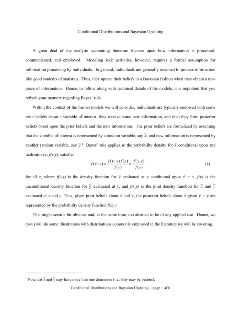
Conditional Distributions and Bayesian Updating
A great deal of the analytic accounting literature focuses upon how information is processed,
communicated, and employed.
Modeling such activities, however, requires a formal assumption for
information processing by individuals. In general, individuals are generally assumed to process information
like good students of statistics. Thus, they update their beliefs in a Bayesian fashion when they obtain a new
piece of information. Hence, to follow along with technical details of the models, it is important that you
refresh your memory regarding Bayes’ rule.
Within the context of the formal models we will consider, individuals are typically endowed with some
prior beliefs about a variable of interest, they receive some new information, and then they form posterior
beliefs based upon the prior beliefs and the new information. The prior beliefs are formalized by assuming
that the variable of interest is represented by a random variable, say ~x , and new information is represented by
another random variable, say ~y .1 Bayes’ rule applies so the probability density for ~
x conditional upon any
realization y, f(x|y), satisfies
f (x | y) 
f (y | x) f (x) f (x, y)

f (y)
f (y)
(1)
for all x, where f(y|x) is the density function for ~
y evaluated at y conditional upon ~x = x, f(y) is the
unconditional density function for ~
y evaluated at y, and f(x,y) is the joint density function for ~x and ~
y
evaluated at x and y. Thus, given prior beliefs about ~x and ~y , the posterior beliefs about ~x given ~y = y are
represented by the probability density function f(x|y).
This might seem a bit obvious and, at the same time, too abstract to be of any applied use. Hence, we
(you) will do some illustrations with distributions commonly employed in the literature we will be covering.
1
~
~
Note that x and y may have more than one dimension (i.e., they may be vectors).
Conditional Distributions and Bayesian Updating – page 1 of 6
Bernoulli
Many models employ a simple structure in which the variable of interest has two possible outcomes and
the information variable has two possible outcomes (i.e., both are characterized by Bernoulli distributions).
Assume the variable of interest ~x has two possible realizations, s or f, where s > f. Let p denote the prior
probability of s. Assume that the information received by the decision maker is represented by the random
variable ~y , which has two possible outcomes, g or b. Assume that the probability of g conditional upon ~x = s
is qg > .5 and the probability of b conditional upon ~x = f is qb > .5. Characterize the posterior distribution for
~x given the following realizations for ~
y.
a) ~y = g
b) ~y = b
c) In a and b, how do qg and qb capture the quality of the information?
Uniform
Another distribution that is often employed for the variable of interest is the uniform distribution.
Assume the variable of interest ~x is uniformly distributed over the range [0,1]. Assume that the information
received by the decision maker is represented by the random variable ~y , which has two possible outcomes, b
or g.
a) Assume that the probability ~
y = b is 1 if ~x  [0,k] and the probability ~y = g is 1 if ~x  (k,1], where k 
(0,1). Characterize the posterior distribution for ~
x if ~y = g and the posterior distribution for ~x if ~
y = b.
b) Repeat question a assuming that the probability ~y = b is q  (.5,1] if ~x  [0,.5] and the probability ~
y=g
is q if ~
x  (.5,1].
Normal
A final distribution that is employed heavily in the literature is the normal distribution. The normal
distribution is employed because its parameters have nice intuitive interpretations (e.g. it is characterized by
a mean and variance and the variance generally serves as a measure of uncertainty and/or quality of
information). We will consider the bivariate normal case first and then turn attention to the multivariate case.
Conditional Distributions and Bayesian Updating – page 2 of 6
Bivariate Normal
Assume prior beliefs about a variable of interested, ~x , and a forthcoming piece of information, ~y , are
represented as follows: ~x is normally distributed with mean x and variance sx ~
y is normally distributed with
mean y and variance sy, and ~
x and ~y have covariance cxy. Assume that an economic decision maker
observes realization y and updates beliefs about ~x . The decision maker’s posterior beliefs are that ~
x is
normally distributed with mean
x 
cxy
sy
(y   y ) ,
and variance

cxy2 
sx  1
.
 sx sy 
To prove this result, note first that, by definition, the joint density function is
2

 (x   )2
sx sy
(x   x ) (y   y ) (y   y )  


x

 .
f (x, y) 
exp 
 2cxy

2
2
2(sx sy  cxy )  sx
sy
sx
sy
 
2 sx sy  cxy




1
Furthermore, by Bayes’ rule we know f(x|y)  f(x,y) where the factor of proportionality, f(y)-1, is not a
function of x. Therefore, we can work with f(x,y) to derive the conditional density function. Specifically, the
conditional density function must be proportional to

 (x   x )2
sx sy
(x   x ) (y   y )  
exp 
 2cxy


2
2(s x sy  cxy ) 
sx
sx
s y  
2 s x sy  cxy2

1



sy
cxy
cxy2
2
2 
 exp 
(x


)

2(x


)
(y


)

(y


)


x
x
y
y
2
sy
sy2
 
 2(sx s y  cxy ) 
2
 
 
c
  x   x  xy (y   y )  
sy
 
 
 exp  

2

cxy 


2s x  1 



sx sy 



2
 
 
cxy
  x  x 
(y   y )  
sy
 
1
 

exp 
.

cxy2 

cxy2 


2s x  1 
2 sx  1 




s
s


sx sy 
x y



Conditional Distributions and Bayesian Updating – page 3 of 6
Note that this last line is the density function for a normally distributed random variable ~
x with the asserted
mean and variance.
To see if you can apply this result consider the following structures and derive the posterior density for ~x
conditional upon ~
y = y.
a) ~x is normally distributed with mean x and variance sx. ~y =x~ +~ where ~ is normally distributed with
mean 0 and variance s. Also, ~
x and ~ are independent.
b) ~x is normally distributed with mean x and precision hx. ~y =x~ +~ where ~ is normally distributed with
mean 0 and precision h. (Note: the precision is the inverse of the variance h = s–1.)
c) ~x = ~y + ~z , where ~
y is normally distributed with mean y and variance sy, ~z is normally distributed with
mean z and variance sz, and ~y and ~z are independent.
Multivariate Normal
~
We can extend the bivariate normal case to multivariate normal distributions. Assume that X is an m
~
variate normal with mean vector x and Y is a n variate normal with mean vector My. Let the covariance
~
~
matrix for X and Y be denoted as
 Sx
C
 yx
C xy 
Sy 
~
~
where Sx is the covariance matrix for X, Sy is the covariance matrix for Y, and Cxy is the covariance matrix
~
~
across the elements of X and Y and Cyx is the transpose of Cxy. The decision maker’s posterior distribution for
~
~
~
X given Y = Y is that X is an m variate normal with mean
 x  C xy Sy1 (Y   y ) ,
and variance
Sx  C xy Sy1C yx ,
where the superscript – 1 denotes the inverse of the matrix.
The proof is analogous to the proof in the bivariate case and is omitted. To make the statement more
concrete, however, we will provide a specific example. Consider a case where the variable of interest is
represented by the random variable ~x and the decision maker obtains two pieces of information represented
Conditional Distributions and Bayesian Updating – page 4 of 6
by the random variables ~y and ~z . Denote the mean and variance of random variable i as I and si
respectively. Denote the covariance between variables i and j as cij. The covariance matrix is
 sx

 cxy
 cxz

cxy
sy
cyz
cxz 

cyz 
sz 
To see the mapping between this matrix and the generic matrix, substitute sx in for Sx,
cxy
cxz 
 sy
c
 yz
cyz 
sz 
in for Cxy and
in for Sy. Applying the formula, the distribution for the variable of interest ~x conditional on realizations y and
z is normal with mean
x 
s c
z xy
 cxz cyz
s y sz  c
2
yz
(y   )  s c
y xz
y
 cxy cyz
s y sz  c
2
yz
(z   ) ,
z
and variance
sx sy sz  sx cyz2  sy cxz2  sz cxy2  2cxy cxz cyz
sy sz  cyz2
.
To test your ability to apply the formula, derive the posterior expectation and variance for ~x conditional
on realizations y and z.
a) ~x = ~y + ~z , where ~
y is normally distributed with mean y and variance sy, and ~z is normally distributed
with mean z and variance sz.
~ , where ~x is normally distributed with mean  and variance s , and ~ is normally
b) ~y = ~x + ~ and ~z =x~ +
x
x
~ is normally distributed with mean 0 and variance s , and ~x , ~
distributed with mean 0 and variance s, 

~ are mutually independent.
and 
~ , where ~x is normally distributed with mean  and variance s , and ~ is normally
c) ~y = ~x + ~ and ~z =~ +
x
x
~ is normally distributed with mean 0 and variance s , and ~x , ~
distributed with mean 0 and variance s, 

~ are mutually independent.
and 
Conditional Distributions and Bayesian Updating – page 5 of 6
Summary
Bayesian updating is a common assumption employed in most of the literature we will consider. By
forcing you to work through these notes, I hope you have refreshed your memory regarding Bayesian
updating. Furthermore, by focusing your attention on some commonly used distributions, you should have a
jump on and a reference for subsequent papers we will cover.
Conditional Distributions and Bayesian Updating – page 6 of 6