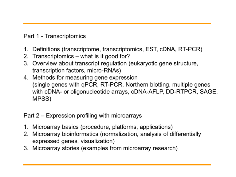
Part 1 - Transcriptomics
1. Definitions (transcriptome, transcriptomics, EST, cDNA, RT-PCR)
2. Transcriptomics – what is it good for?
3. Overview about transcript regulation (eukaryotic gene structure,
transcription factors, micro-RNAs)
4. Methods for measuring gene expression
(single genes with qPCR, RT-PCR, Northern blotting, multiple genes
with cDNA- or oligonucleotide arrays, cDNA-AFLP, DD-RTPCR, SAGE,
MPSS)
Part 2 – Expression profiling with microarrays
1. Microarray basics (procedure, platforms, applications)
2. Microarray bioinformatics (normalization, analysis of differentially
expressed genes, visualization)
3. Microarray stories (examples from microarray research)
Part 1 –
Transcriptomics
(Gene Expression Profiling)
The Language Of Transcriptomics
Genome
= entire DNA sequence of an organism
Transcriptome
= percentage of the genetic code that is transcribed into RNA molecules
(depends on development, environment, time of the day, tissue)
= collection of all gene transcripts present in a given cell/tissue at a given
time (“snapshot”)
Transcriptomics
= global analysis of gene expression = genome-wide expression profiling
cDNA
= complementary DNA synthesized from mature mRNA by the enzyme
reverse transcriptase
cDNA library
= a population of bacterial transformants or phage lysates in which each
mRNA isolated form an organism or tissue is represented as its cDNA
insertion in a plasmid or a phage vector
The Language Of Transcriptomics
RT-PCR
= a one or two-step process for converting mRNA to cDNA and the
subsequent amplifcation of the reversely-transcribed DNA by PCR
EST (Expressed Sequence Tag)
= small pieces of DNA (200 - 500 bp) generated by sequencing either one
or both ends (5’EST and 3’EST) of an expressed gene (cDNA)
= can be used to identify unknown genes and to map their positions within
a genome
Hybridization
= based on complementary molecules, sequences that are able to basepair with one another. Adenine is the complement of thymine, guanine is
the complement of cytosine. Therefore, the complementary sequence to GT-C-C-T-A will be C-A-G-G-A-T. When two complementary sequences find
each other, they will lock together, or hybridize.
The Language Of Transcriptomics
PCR (Polymerase chain reaction)
= technique that results in the exponential amplification of almost any
region of a selected DNA molecule
= repeated cycles of denaturation,
annealing and extension with the
amount of DNA template doubling
during each cycle
The –omics World
Genomics
(Genome)
DNA
Genotype
Transcription
mRNA
Transcriptomics
(Transcriptome)
Translation
Protein
provide structure &
drive metabolism
substrate
product
Proteomics
(Proteome)
Metabolomics
(Metabolome)
Phenotype
morphology
physiology
behaviour
ecology
Common to all -omics: global (often genome-wide) approaches
What Can We Learn From Transcriptomics?
 get an understanding of genes and pathways involved in
biological processes (“guilt by association”: genes with similar
expression may be functionally related and under the same
genetic control mechanism)
 help elucidating the function of unknown genes based on their
spatial and temporal expression
 identifies marker genes for diagnosis of diseases
gene expression is a proxy for cis- and trans- regulation
(allows indirect inferences about genetic differences)
 may be a proxy for changes in the proteome and metabolome
Transcriptomics –
Regulation of Transcription
Structure Of A Eukaryotic Gene
Transcribed region
5’ end of gene
Upstream
regulatory
region
5’ untranslated
region of mRNA
3’ end of gene
Coding sequence
ORF (open reading frame)
3’ untranslated
region of mRNA
Promoter
+1
enhancers
e.g. ERE
CAAT TATA
Transcription start
AUG Exon Intron Exon Intron Exon
Ter
Initiator
Terminator codon
codon
UGA, UAA or UAG
Basic promoter sequence motifs such as TATA and CAAT, additional promoter elements
such as ERE (ethylene response element, in some plant genes) and up- or downstream
regulatory regions on the same strand as the coding region are called cis-elements.
Before the RNA transcript (mRNA) serves as a template for protein biosynthesis, noncoding sequences (introns) are eliminated, coding sequences (exons) are fused (referred
to as ‘splicing’) and the 5‘ and 3‘ untranslated regions (UTRs) are post-transcriptionally
modified. Open reading frames (ORFs) that are translated into a protein always start with
the initiator codon AUG and end with one of the terminator codons UGA,UAA or UAG.
Regulation Of Transcript Abundance By …
…transcription factors
Close-up of the promoter of the plant gene strictosidine
synthase (alkaloid synthesis)
Cis - acting elements
-339
-208
BA
-108
-103 -100
G-Box
CrBPF1
-58
JERE
CrMyc2 CrGBFs ORCAs
+1
TATA
STR gene
RNA
polymerase II
Trans - acting factors (= transcription factors)
DNA binding proteins that activate or
suppress transcription and thus modulate
transcript abundance
Regulation Of Transcript Abundance By MicroRNAs
= miRNAa = small, single-stranded RNA molecules (~21-mer) that bind to
complementary of one or more mRNAs (often transcription factor mRNAs)
miRNA – RISC
complex binding to
complementary
mRNA
Mature miRNA within
RNA-induced silencing
complex (RISC)
miRNAs either degrade or impair the
translation of their target mRNAs!
Taken from http://www.ambion.com/techlib/resources/miRNA/index.html
4 Hypothetical Scenarios Of Gene Regulation
activator
act
suppressor
+
red gene
sup
microRNA gene
red gene transcript
X
act
act
X
red gene
red gene
cis-mutation
X
trans-mutation
activator
cis-mutation in activator
red gene
sup
X
cis-mutation in miRNA
microRNA gene
microRNA transcript
activator
activator transcript
degradatin of activator transcript
activator
missing
red gene
Transcriptomics –
Methods For Measuring
Gene Expression
Methods To Detect Single Gene Transcriptional Changes
Northern Blotting
 transcript-specific
radioactive probes
are used to identify a
target mRNA species
within an immobilized
RNA sample
PCR-based
 based on the ability of a PCR to exponentially amplify initial
differences in transcript number
 amplified products are visualized either in real time during
(qPCR, A) or after (RT-PCR, B) the reaction
A
ΔRn
Hybridizationbased
B
M.s.-induced - local
M.s.-induced - systemic
Control
T. urticae
1d
1d
3d
3d
PR2
Control - local
Control - systemic
SAMS
SAMDC
threshold
probe
ACO
CT
cycles
rRNA
RWC L C
14.2
Reporter gene-based
23.5
 fusions of a promoter of a gene of interest
with a reporter gene: b-glucuronidase
(GUS), green fluorescent protein, luciferase
 reporter activity is measured
histochemically or by fluorescence or
luminescence
 allows for detailed spatial and kinetic
analyses of transcript accumulation
39.1
41.6
61.1
68.1
18 S
Proof of a herbivore-responsive
promoter by GUS staining
Larvaeattacked
Control
Methods To Detect Multiple Gene Transcriptional Changes
PCR-based: Differential Display RT-PCR, cDNA-AFLP
 reverse transcription of mRNA into cDNA
 divide cDNA pool into subsets by selective PCR amplification
 separation of subpools on high resolution gels
 quantification of band intensity
Hybridization-based: Macroarrays, microarrays
 a small membrane (macroarray) or glass slide (microarray) containing samples
of many genes arranged in a regular pattern
 mRNA samples of interest are fluorescently labelled and either singly or
competitively hybridized to a slide
 in a single experiment, the expression levels of thousands of genes can be
determined by measuring the amount of mRNA bound to each gene on the array
Sequencing-based: SAGE (Serial Analysis of Gene Expression)
MPSS (Massively Parallel Signature Sequencing)
 short sequence signatures produced from a defined position within an mRNA
 the relative abundance of these signatures (tags) in a given library represents
a quantitative estimate of expression of that gene
 no sequence knowledge required! universal platform to study any transcript
Sequencing-Based Methods To Detect Multiple Changes
SAGE
 concatemerized tags are sequenced using a
traditional automated DNA sequencing method
 tags are ~9 to 14 bp in length
 library may contain ~50,000 tags
MPSS
 uses a novel sequencing method whereby
thousands of sequences are obtained
simultaneously by sequencing off of beads
 tags are 17-21bp in length
 library may contain about 4 million tags
Solexa (purchased by AWC!)
 uses a novel sequencing method whereby
thousands of sequences are obtained
simultaneously by sequencing off of clusters
within a flow cell
 tags are 17bp in length
 one lane in a flow cell may yield more than
6 million tags
SAGE procedure
Part 2 –
Expression Profiling With
Microarrays
Microarray Basics
Gene Probes
(cDNAs, ESTs, oligos)
Technologies:
Healthy tissue
Diseased tissue
mRNA
mRNA
cy3-labeled
cDNA
cy5-labeled
cDNA
 robotic spotting (ESTs,
oligonucleotides)
 in-situ synthesis
(oligonucleotides),
Affymetrix, NimbleGen,
Agilent
Hybridization:
 competitive in two
color arrays
 single in one color
arrays
Cy signal ~ amount of mRNA in healthy & diseased tissue
Green spots = cDNA from healthy tissue hybridized to the target DNA
Red spots = cDNA from diseased tissue hybridized to the target DNA
Yellow spots = control and sample cDNA hybridized equally to the
target DNA
Blue spots = neither control nor sample cDNA hybridized to the target
DNA
Cross-Species
Hybridization:
 Gene probes and
samples originate from
different species
Microarray Applications
Medicine
 Disease-associated expression patterns (diagnosis)
 Cell-cycle monitoring (cancer research)
 Treatment-induced expression pattern (drug development and response)
Biology
 Development and Morphology (juveniles vs adults, male vs female,
tissue 1 vs tissue 2)
 Interactions between organisms (antagonistic, mutualistic, competitive)
and organisms and their environments (temperature, radiation, draught,
nutrient levels, toxins and heavy metals)
 Evolution (within- and between species variation, hybrids vs parents,
diploids vs polyploids)
 Functional analyses (wild type vs mutant)
 Time series
Microarray Stories – Examples From Biology
Hybrid sunflowers colonizing new habitats…
Lai et al., Molecular Ecology 2006
 26 lower and 32 higher expressed genes in the hybrid sunflower
Helianthus deserticola when compared with its two parental species,
H. annuus and H. petiolaris,
 Among them many transport-related genes that may be important
in the desert environment (acting in preventing desiccation)
 Differentially expressed genes are candidates for ecological
divergence
Source: Rieseberg lab
website
Tobacco plants perceiving chemical cues in caterpillar saliva…
Halitschke et al., Plant Physiology 2003
 majority of the genes up- and
downregulated in tobacco when treated
with caterpillar saliva were also induced
with only two compounds isolated from
saliva (fatty-acid amino acid conjugates)
 tobacco responds differently to
mechanical wounding than to caterpillar
attack because of these compounds
Caterpillar spit
Chemical cue
Caterpillar
spit
Chemical
cue
Microarray Stories – Examples From Biology
Behavioural plasticity in honeybees…
Whitfield et al., Science 2003
 Transition of adult honeybees from hive
work to foraging is associated with mRNA
abundance in the brain
 Individual brain expression profiles can
reliably predict the behaviour of a bee
based on as little as ten predictor genes
Nightshade and tobacco respond differently to a common herbivore…
Schmidt et al., The Plant Journal 2005
 Venn diagram of the numbers of
overlapping and non-overlapping up- and
down-regulated genes in two plant
species of the nightshade family that are
induced by tobacco hornworm feeding
 no “blue print” of defence responses,
evolutionary history matters!
Steps In A Microarray Experiment
Question-driven
 Goals? Hypotheses? Questions?
Platform
 What technology? Source of gene probes?
 Cross-species hybridization?
Experimental design
 Replication level
 Hybridization scheme
 What statistics, what analysis software?
Laboratory steps
 Sample preparation and labelling
 Hybridization (manual or robotic) and washing
 Image acquisition (Scanner with two lasers)
Bioinformatic steps
 Data transformation and normalization
 Analysis of differentially expressed genes
(multiple testing issue, multivariate statistics, gene ontology)
 Visualization (graphics)
 Data storage (databases, MIAME standards)
Data interpretation
 Answers? New Hypotheses? Follow-up experiments?
 Validation?
Microarray Bioinformatics –
Data Pre-Processing
Data Pre-Processing – Overview
Resolves systematic errors and bias introduced by experimental platform
1. Data cleaning and transformation
(removing flagged spots, background subtraction, taking logarithms)
2. Within-array normalization
(removes dye and spatial bias, brings cy3 and cy5 channels on equal
footing)
 linear regression of cy5 against cy3 (scatter plots)
 linear/non-linear regression of log ratios against average log
intensity (MA plots)
3. Between-array normalization
(enables comparison of multiple arrays, brings samples hybridized to
different arrays on equal footing, box plots)
 Scaling, Centering, Distribution normalization (quantile)
Transformation – Taking Logarithms (log (to base 2))
Cy3 = green (sample 1), Cy5 = red (sample 2)
Cy5 > Cy3 = higher expression in sample 2
Cy5 < Cy3 = higher expression in sample 1
Cy5 = Cy3 = equal expression in both samples
M (log fold ratio) = log2(cy5/cy3) = log2(cy5) – log2(cy3)
A (average log intensities) = (log2(cy5) + log2(cy3))/2
Log fold ratios have a natural symmetry which
reflects the biology that is not present in the
raw fold difference:
2 fold up- and down-regulated genes have a raw
fold difference of 2 and 0.5 and non-regulated
genes have a raw fold difference of 1. On the log2
scale 2 fold up- and down-regulated genes
correspond to log fold ratios of +1 and -1 and
non-regulated genes have a log fold ratio of 0.
cy5/cy3
log2 (cy5/cy3)
Transformation – Taking Logarithms (log (to base 2))
scatter plot
Raw intensities are not
evenly distributed across the
intensity range, variability of
the data increases with
intensity and distributions of
raw intensities are right
skewed in both channels
(Cy3 and Cy5)
Cy5 raw intensity
before
histogram
Cy3 raw intensity
Cy3 raw intensity
Cy5 raw intensity
The data is spread evenly
across the intensity range
and the variability is the
same at most intensities,
plus the intensity
distributions are closer to
a bell-shaped normal
curve.
Cy5 log intensity
after
Cy3 log intensity
Cy3 log intensity
Cy5 log intensity
Within Array Normalization – MA Plots & Regression
X-axis = average of cy3 and cy5 log intensities (A)
Y-axis = difference between cy5 and cy3 log intensities, log fold ratio (M)
Log fold ratio
Non-linear regression (loess)
Loess normalized
Log fold ratio
after
Linear normalized
Log fold ratio
before
Log fold ratio
Linear regression
Average log intensity
Between Array Normalization – Box Plots
Log fold ratio
whiskers = outliers or extreme values
central line = mean or median
box = standard deviation or middle
50% of the data
Scaling
 subtracting the mean
 equalizes the mean across all
samples
Distribution normalization
Distributionnormalized log ratio
Scaled log ratio
Centered log ratio
Centering
 subtracting the mean + dividing by  data distributions of all
arrays are identical (quantile
standard deviation (sd)
normalization)
 equalizes mean and sd
Microarray Bioinformatics –
Analysis Of Differentially
Expressed Genes
Two Questions A Microarray Experiment Should Answer…
1. Which genes are differentially expressed in one set of samples
relative to another?
Comparing 2 samples
 Parametric statistics (one-sample t-test, two-sample t-test)
 Non-parametric statistics (Wilcoxon sign-rank test, Mann Whitney test)
 Bootstrap analyses
Comparing >2 samples and/or measuring response to more than one variable
 One-way ANOVA, multifactor ANOVA
 General Linear Models
 Bootstrap analyses
Mulitplicity of testing
 False Discovery Rate, Bonferroni correction
2. What are the relationships between genes or samples being measured?
Dimensionality reduction
 Principal components analysis (PCA), multidimensional scaling (MDS)
Grouping of genes or samples
 Hierarchical clustering
 K-means clustering, Self-organizing maps
 Bootstrap analyses
Analysis Of Differentially
Expressed Genes –
Which genes are differentially expressed in one
set of samples relative to another?
Hypothesis Testing: T-test and P-value
Each hypothesis test builds a probabilistic model under the null hypothesis that
there is no biological effect. Using this model it is possible to calculate the probability
of observing a statistic that is at least as extreme as the observed statistic in the
data (= p-value). Usually, a p<0.05 is considered small enough to reject the null
hypothesis. P-values are also know under type 1 error – the probability of rejecting
the null hypothesis when it is actually true (= false positives).
Example: unpaired t-test
Null hypothesis (H0): gene x is not differentially expressed between A patients and B
patients
1. Calculate the t-statistic for gene x
(incorporates mean, standard deviation
and sample size of both A and B
patients)
2. Compare t-statistic with a t-distribution
with an appropriate number of degrees
of freedom (df)
3. If t-statistic is more extreme than the
critical t-statistic at a chosen
significance level (e.g. p=0.05) reject the
null hypothesis, otherwise accept it
T-distribution (df, p=0.05)
Hypothesis Testing: Bootstrap Test
Example: bootstrap test
Null hypothesis (H0): gene x is not differentially expressed between A patients
and B patients
1. generate many random data sets by
re-sampling the original data, each
individual is randomly allocated a
measurement from either group
2. compare some property of the real
data (e.g. t-statistic) with the
distribution of the same property in
the random data sets
3. compute proportion of t-statistics that
have a more extreme value than the
t-statistic from the real data (=pvalue)
4. small p-value indicates differential
expression of gene X
Distribution of bootstrap t-statistics
t-statistic of
real data
majority of bootstrap statistics are less
extreme then the real statistic (p<0.001)
Bootstrapping works for paired and unpaired analyses, ANOVA and Cluster
analysis, is robust and powerful, but computationally intensive!
Multiplicity of Testing
Meaning of a p-value? P-value of 0.01 means a false positive rate of 1%.
Calculating the false discovery rate in a microarray experiment
Imagine an array with 6350 genes and an experiment where 184 genes are
differentially expressed at p=0.01. That means 64 genes would be expected to
appear differentially expressed even when they’re not (false discovery rate 35%).
With decreasing p-value, the false discovery rate also decrease, but so does the
number of differentially expressed genes – choose a p-value which balances
number of differentially expressed genes and false discovery rate!
False discovery
rate
Fine print: Alternatively – multiply each p-value by the number of genes in the analysis to
obtain Bonferroni-adjusted p-values. Usually none of the adjusted p-values is significant,
thus Bonferroni correction is too stringent for microarray analyses!
The Volcano Plot Arranges Genes …
... along dimensions of biological and
statistical significance:
The log fold change is plotted on the
x-axis while the y-axis represents
statistical evidence (either a p-value
on a negative log scale – so smaller
p-values appear higher up or an
odds ratio on a positive log scale –
so higher odds ratios appear higher
up).
The x-axis indicates biological
impact of the change; the y-axis
indicates the reliability of the change.
The researcher can then make
judgements
about
the
most
promising candidates for follow-up
studies, by trading off both these
criteria.
Example. Up (red) and down (green) regulated
genes in a tobacco plant attacked by a caterpillar
as compared to an un-attacked plant on a 1.5fold
change level (-0.58 and +0.58 on log scale). Black
genes either have a too low log fold change or log
odds ratio or both.
Analysis of Differentially
Expressed Genes –
What are the relationships between genes or
samples being measured?
Dimensionality Reduction
Methods for visualizing high-dimensional microarray data in two or three
dimensions: Principal Components Analysis (PCA)
PCA projects highdimensional space into twodimensional space by
capturing as much of the
variability of the original data
as possible
5h
2h
7h
9h
 starts with a variance-covariance
matrix of all genes
 calculates new variables that each
explain a portion of the variance
(=principal components)
Example: Six arrays representing
six time points during yeast
sporulation
0.5h
11h
 three late samples fairly similar, main changes
occur over first 7 h
 plus some processes switched on after the first
5h and then switched off
Dimensionality Reduction
Methods for visualizing high-dimensional microarray data in two or three
dimensions: Multidimensional Scaling (MDS)
MDS locates profiles in two-dimensional space such that their distances are
as close as possible to their distances in the higher dimensional space
 starts by calculating the distance between profiles
 distance measures can vary (Euclidean distance, Pearson correlation, Spearman correlation)
Example: Six arrays representing six time points during yeast sporulation
a) using Euclidean distance
b) using Pearson Correlation
5h
2h
2h
7h
9h
7h
9h
0.5h
5h
11h
0.5h
11h
Hierarchical Clustering…
…arranges gene and/or sample profiles into a tree so that similar
profiles are closer together and dissimilar profiles are farther apart.
How it’s done:
1. Calculate distance matrix between genes/samples (different methods)
2. Find nearest entries in distance matrix and join them into a cluster
3. Compute the distance between the newly formed cluster and the other
genes/samples and clusters (different methods)
4. Return to step 1 until all genes and clusters are linked
Results vary depending on choice of distance metric and cluster linkage!
Pearson correlation +
single linkage
Pearson correlation +
complete linkage
Pearson correlation +
average linkage
From Hierarchical Clustering To Heatmaps
Heatmap
 false color image with a dendrogram added on top and on the side
 very frequently used for visualization of microarray results
top dendrogram represents relations between
samples (e.g. patients or time points)
Side dendrogram
represents relations
between genes
Microarray Data Interpretation – Gene ontology (GO)
Output of a microarray analysis:
List of differentially expressed genes, annotated mostly with their names
– not helpful for biological interpretation!
Gene Ontology Consortium developed three structured vocabularies
(ontologies) that describe gene products in terms of their associated
biological processes, cellular components and molecular functions in
a species-independent manner.
For example, the gene product cytochrome c can be described by the:
 molecular function term oxidoreductase activity,
 biological process terms oxidative phosphorylation and induction of
cell death,
 cellular component terms mitochondrial matrix and mitochondrial
inner membrane.
GO is constantly up-dated (http://www.geneontology.org/) and a
very valuable tool for micorarray data interpretation!
For more information:
Microarray case studies:
• Halitschke, R., K. Gase, D. Q. Hui, D. D. Schmidt, and I. T. Baldwin. 2003. Molecular interactions
between the specialist herbivore Manduca sexta (Lepidoptera, Sphingidae) and its natural host
Nicotiana attenuata. VI. Microarray analysis reveals that most herbivore-specific transcriptional
changes are mediated by fatty acid-amino acid conjugates. Plant Physiology 131:1894-1902.
• Lai, Z., B. L. Gross, Y. Zou, J. Andrews, and L. H. Rieseberg. 2006. Microarray analysis reveals
differential gene expression in hybrid sunflower species. Molecular Ecology 15:1213-1227.
• Whitfield, C. W., A. M. Cziko, and G. E. Robinson. 2003. Gene expression profiles in the brain
predict behavior in individual honey bees. Science 302:296-299.
• Schmidt, D. D., C. Voelckel, M. Hartl, S. Schmidt, and I. T. Baldwin. 2005. Specificity in ecological
interactions. Attack from the same lepidopteran herbivore results in species-specific transcriptional
responses in two solanaceous host plants. Plant Physiology 138:1763-1773.
Microarray text books:
• Stekel, D., ed. 2003. Microarray Bioinformatics. Cambridge University Press, Cambridge.
• Draghici, S., ed. 2003. Data Analysis Tools for DNA Microarrays. Chapman & Hall/CRC, Boca
Raton.
Microarray freeware:
http://www.r-project.org/ + http://www.bioconductor.org/
Microarray online info:
http://www.ncbi.nlm.nih.gov/About/primer/microarrays.html
Solexa sequencing:
http://www.illumina.com/morethansequencing/Technology.ilmn