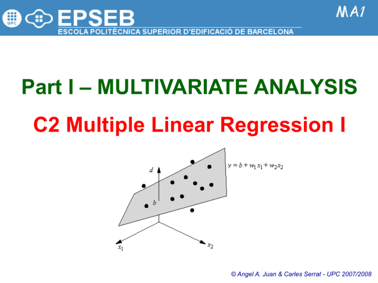
Part I – MULTIVARIATE ANALYSIS
C2 Multiple Linear Regression I
© Angel A. Juan & Carles Serrat - UPC 2007/2008
1.2.1: The t-Distribution (quick review)

The t-distribution is basic to statistical inference.

The t-distribution is characterized by the degrees of
freedom parameter, df.

For a sample of size n  df = n-1

Like the normal, the t-distribution is symmetric, but it is
more likely to have extreme observations.
As the degrees of freedom
increase, the t-distribution
better approximates the
standard normal.
1.2.2: The F-Distribution (quick review)

The F-distribution is basic to regression and analysis
of variance.

The F-distribution has two parameters: the numerator,
m, and denominator, n, degrees of freedom  F(m,n)

Like the chi-square distribution, the F-distribution is
skewed.
1.2.3: The Multiple Linear Regression Model

Multiple linear regression analysis studies how a dependent
variable or response y is related to two or more independent
variables or predictors, i.e., it enables us to consider more
factors –and thus obtain better estimates– than simple linear
regression.
Independent
variables
Error
term
y   0   1 x1   2 x 2  ...   P x P  

Multiple Linear Regression Model (MLRM):

In general, the regression model parameters will not be
known and must be estimated from sample data.

Estimated Multiple Regression Equation:
Parameters (unknown)
yˆ  b0  b1 x1  b2 x 2  ...  b P x P
Estimate for y
Parameters’ estimates

The Least squares method uses sample data to provide the
values of b0, b1, b2, …, bp that minimize the sum of squared
residuals –the deviations between the observed values, yi,
and the estimated ones:
2
ˆ
m in   y i  y i 
We will focus on how to
interpret the computer
outputs rather than on
how to make the multiple
regression calculations.
1.2.4: Single & Multiple Regress. (Minitab)

File: LOGISTICS.MTW

Stat > Regression >
Regression…
Managers of a
Logistics company
want to estimate the
total daily travel time
for their drivers.
At the 0.05 level of significance, the t value of 3.98 and its corresponding
p-value of 0.004 indicate that the relationship is significant, i.e., we can
reject H0: β1 = 0. The same conclusion is obtained from the F value of
15.81 and its associated p-value of 0.004. Thus, we can reject H0: ρ = 0
and conclude that the relationship between Hours and Km is significant.
In MR analysis, each
regression coefficient
represents an estimate of
the change in y
corresponding to a one
unit change in xi when all
other independent
variables are held constant;
e.g.: 0.0611 hours is an
estimate of the expected
increase in Hours
corresponding to an
increase of one Km when
Deliveries is held
constant.
66.4% of the variability in Hours can be explained by
the linear effect of Km.
1.2.5: The Coefficient of Determination (R2)

The total sum of squares (SST) can be partitioned
into two components: the sum of squares due to
regression (SSR) and the sum of squares due to
error (SSE):
The value of SST is the
same in both cases, but
SSR increases and SSE
decreases when a
second independent
variable is added  The
estimated MR equation
provides a better fit for
the observed data.


y
 y 
2
i
SST

  yˆ
 y 
2
i

SSR
SST = 23.900
SSR = 15.871
SSE = 8,029
The multiple coefficient of determination, R2 = SSR /
SST, measures the goodness of fit for the estimated
MR equation.
R2 can be interpreted as the proportion of the
variability in y that can be explained by the estimated
MR equation.
y
i
 yˆ i 
SSE
SST = 23.900
SSR = 21.601
SSE = 2,299
R 
2
SSR
SST
R2 always increases as new independent
variables are added to the model. Many
analysts prefer adjusting R2 for the number
of independent variables to avoid
overestimating the impact of adding new
independent variables.
2
1.2.6: Model Assumptions


General assumption: The form of the model is
correct, i.e., it’s appropriate to use a linear
combination of the predictor variables to predict the
value of the response variable.
Assumptions about the error term ε:
1.
The error ε is a random variable with E[ε] = 0
2.
Var[ε] = σ2 and is constant for all values of the
independent variables x1, x2, …, xp
3.
The values of ε are independent
4.
ε is normally distributed and it reflects the deviation
between the observed values, yi, and the expected
values, E[yi]

Any statement about hypothesis tests or confidence
intervals requires that these assumptions be met.

Since the assumptions involve the errors, and the
residuals, yobserved – yestimated, are the estimated
errors, it is important to look carefully at the
residuals.
This implies that, for given values of x1, x2, …,
xp, the expected value of y, E[y], is given by
E[y] = β0 + β1x1 + β2x2 + … + βpxp
This implies that Var[y] = σ2,
and it is also constant.
i.e.: the size of the error for a particular set of
values for the predictors is not related to the
size of the error for any other set of values.
This implies that, for the given values
of x1, x2, …, xp, the response y is also
normally distributed.
The errors do not have to
be perfectly normal, but
you should worry if there
are extreme values:
outliers can have a major
impact on the regression.
1.2.7: Testing for Significance

In SLR, both the t test and the F test
provide the same conclusion (same
p-value)

In MLR, both tests have different
purposes:
1.
2.
1. Since pvalue < α  a
significant
relationship is
present
between the
response and
the set of
predictors.
The F test is used to determine the MS 2Error provides an unbiased estimate
of σ , the variance of the error term
overall significance, i.e., whether
there is a significant relationship
between the response and the set of
all the predictors.
If the F test shows an overall
significance, then separated t tests
are conducted to determine the
individual significance, i.e., whether
each of the predictors is significant.
H 0 : i  0
t t est for the i th param eter: 
H1 : i  0
T est S tatistic : t 
C oef i
S E C oe f i
2. Also, since
p-value < α 
both predictors
are statistically
significant.
If an individual parameter is not significant, the corresponding
variable can be dropped from the model. However, if the t test shows
that two or more parameters are not significant, no more than one
variable can ever be dropped: if one variable is dropped, a second
variable that was not significant initially might become significant.
 H 0 :  1   2  ...   p  0
F test: 
 H 1 : O ne or m ore of the param eters is not ze ro
S S R eg
T est S tatistic: F 
M S R eg
M S E rr

p
S S E rr
( n - p - 1)
 n  # observ.

 p  # predictors
1.2.8: Multicollinearity

Multicollinearity means that some predictors are
correlated with other predictors.

Rule of thumb: multicollinearity can cause problems if
the absolute value of the sample correlation
coefficient exceeds 0.7 for any two independent
variables.

Potentials problems:


In t tests for individual significance, it is possible to
erroneously conclude that none of the individual
parameters are significantly different from zero when
an F test on the overall significance indicates a
significant relationship.

It results difficult to separate the effects of the
individual predictors on the response.

Severe cases could even result in parameter estimates
(regression coefficients) with the wrong sign.
Possible solution: to eliminate predictors from the
model, especially if deleting them has little effect on
R2.
Predictors are also called independent
variables. This does not mean, however,
that predictors themselves are
statistically independent. On the contrary,
predictors can be correlated with one
another.
Does this mean that no predictor
makes a significant contribution to
determining the response?
No, what this probably means is
that with some predictors
already in the model, the
contribution made by the others
has been already included in the
model (because of the correlation).
1.2.9: Estimation & Prediction

Given a set of values x1, x2, …, xp, we can
use the estimated regression equation to:
a)
b)


Estimate the mean value of y associated
to the given set of xi values
Predict the individual value of y associated
to the given set of xi values
Both point estimates provide the same
result.
yˆ  Eˆ  y   b0  b1 x1  b2 x 2  ...  b P x P
Given x1, x2, …, xp, the point estimate of an
individual value of y is the same as the
point estimate of the expected value of y
Given Km = 50 and Deliveries = 2
 point estimate for y = point
estimate for E[y] = 4.035
Point estimates do not provide any idea of
the precision associated with an estimate.
For that we must develop interval
estimates:

Confidence interval: is an interval estimate
of the mean value of y for a given set of xi
values

Prediction interval: is an interval estimate
of an individual value of y corresponding to
a given set of xi values
Confidence Intervals for E[y] are
always more precise (narrower)
than Prediction Intervals for y.
1.2.10: Qualitative Predictors

A regression equation could have
qualitative predictors, such as gender
(male, female), method of payment (cash,
credit card, check), and so on.

If a qualitative predictor has k levels, k – 1
dummy variables are required, with each of
them being coded as 0 or 1.

File: REPAIRS.MTW
Repair time (Hours) is
believed to be related to two
factors, the number of
months since the last
maintenance service
(Elapsed) and the type of
repair problem (Type).
Since k = 3 (software,
hardware and firmware),
we had to add 2 dummy
variables
We could try to eliminate non-significant
predictors from the model and see what happens…
1.2.11: Residual Analysis: Plots (1/2)

The model assumptions about the error term, ε,
provide the theoretical basis for the t test and
the F test.

The residuals provide the best information
about ε; hence an analysis of the residuals is
an important step in determining whether the
assumptions for ε are appropriate.
R esidual for observation i :
ri  y i  yˆ i  y i  E  y i    i

The standardized residuals are frequently used
in residuals plots and in the identification of
outliers.

Residual plots:
1.
2.
If these assumptions appear questionable,
the hypothesis tests about the significance of
the regression relationship and the
interval estimation results may not be valid.
Standardized residuals against predicted
values: this plot should approximate a
horizontal band of points centered around 0. A
different pattern could suggest: (i) that the
model is not adequate, or (ii) a non-constant
variance for ε
Normal probability plot: this plot can be used to
determine whether the distribution of ε appears
to be normal
S tandardized residual for observation i :
sri 
ri  E  ri 
s ri

ri
s ri
( s ri  standard deviation of resiudal i )
A linear model is
not adequate
Non-constant
variance
1.2.11: Residual Analysis: Plots (2/2)

File: LOGISTICS.MTW

Stat > Regression >
Regression…
R e s idua ls V e r s us the F itte d V a l ue s
(r e s po ns e is Ho ur s )
S t a nd a r d iz e d R e s id ua l
2
The plot of standardized residuals against predicted
values should approximate a horizontal band of points
centered around 0. Also, the 68-95-99% rule should apply.
In this case, the plot does not indicate any unusual abnormalities.
Hence, it seems reasonable to assume constant variance. Also, all
of the standardized residuals are between -2 and +2 (i.e., more
than the expected 95% of the standardized residuals). Hence, we
have no reason to question the normality assumption.
1
0
-1
-2
4
5
6
7
8
9
Fit t e d V a lue
N o r ma l P r o ba bility P lo t o f the R e s idua ls
(r e s po ns e is Ho ur s )
The normal probability plot for the standardized residuals
represents another approach for determining the validity of the
assumption that the error term has a normal distribution. The
plotted points should cluster closely around the 45-degree.
In general, the more closely the points are clustered about the
45-degree line, the stronger the evidence supporting the
normality assumption. Any substantial curvature in the plot is
evidence that the residuals have not come from a normal
distribution.
99
95
90
80
Pe r c e nt
70
60
50
40
30
20
10
5
1
-3
-2
-1
0
S t a nd a r d iz e d R e s id ua l
1
2
3
In this case, we see that the points are grouped
closely about the line. We therefore conclude that the
assumption of the error term having a normal
distribution is reasonable.
1.2.12: Residual Analysis: Influential Obs.

Outliers are observations with larger than average response or predictor values.
It is important to identify outliers because they can be influential observations,
i.e., they can significantly influence your model, providing potentially misleading
or incorrect results.

Apart from residual plots, there are several alternative ways to identify outliers:
1.
Leverages (HI) are a measure of the distance between the x-values for an
observation and the mean of x-values for all observations. Observations with a
HI>3(p+1)/n may exert considerable influence on the fitted value, and thus on the
regression model
2.
Cook's distance (D) , is calculated using leverage values and standardized residuals.
It considers whether an observation is unusual with respect to both x- and y-values.
Geometrically, Cook's distance is a measure of the distance between the fitted values
calculated with and without the observation. Observations with a D>1 are influential
3.
DFITS represents roughly the number of estimated standard deviations that the fitted
value changes when the corresponding observation is removed from the data.
Observations with a DFITS>Sqrt[2(p+1)/n] are influential
Minitab identifies observations with a
large leverage value with an X in the
table of unusual observations.
1.2.13: Autocorrelation (Serial Correlation)

Often, the data used for regression studies are
collected over time. In such cases,
autocorrelation or serial correlation can be
present in the data.

Autocorrelation of order k: the value of y in time
period t is related to its value in time period t-k.

The Durbin-Watson statistic, 0<=DW<=4, can
be used to detect first-order autocorrelation:


If DW close to 0  positive autocorrelation
(successive values of the residuals are close
together)

If DW close to 4  negative autocorrelation
(successive values of the residuals are far
apart)

If DW close to 2  no autocorrelation is
present
Including a predictor that measures the time of
the observation or transforming the variables
can help to reduce autocorrelation.
When autocorrelation is present, the
assumption of independence is violated.
Therefore, serious errors can be made in
performing tests of statistical significance
based upon the assumed regression model
The Durbin-Watson test for autocorrelation
uses the residuals to determine whether firstorder autocorrelation is present in the data.
The test is useful when sample size >= 15