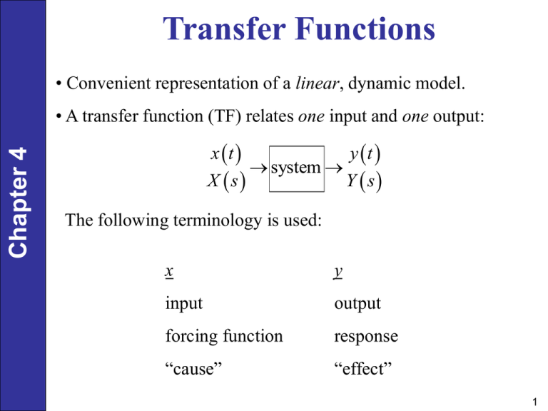
Transfer Functions
• Convenient representation of a linear, dynamic model.
Chapter 4
• A transfer function (TF) relates one input and one output:
x t 
y t 
 system 
X s
Y s
The following terminology is used:
x
y
input
output
forcing function
response
“cause”
“effect”
1
Definition of the transfer function:
Chapter 4
Let G(s) denote the transfer function between an input, x, and an
output, y. Then, by definition
G s
Y s
X s
where:
Y s
L  y  t  
X s
L  x  t  
2
Development of Transfer Functions
Chapter 4
Example: Stirred Tank Heating System
Figure 2.3 Stirred-tank heating process with constant holdup, V.
3
Recall the previous dynamic model, assuming constant liquid
holdup and flow rates:
dT
V C
 wC Ti  T   Q
dt
(1)
Chapter 4
Suppose the process is initially at steady state:
T  0   T , Ti  0   Ti , Q  0   Q
 2
where T steady-state value of T, etc. For steady-state
conditions:
0  wC Ti  T   Q
(3)
Subtract (3) from (1):
dT
V C
 wC Ti  Ti   T  T     Q  Q 
dt
(4)
4
But,
dT d T  T 

because T is a constant
dt
dt
(5)
Chapter 4
Thus we can substitute into (4-2) to get,
dT 
V C
 wC Ti  T    Q
dt
(6)
where we have introduced the following “deviation variables”,
also called “perturbation variables”:
T  T  T , Ti Ti  Ti , Q Q  Q
(7)
Take L of (6):
V C  sT   s   T   t  0   wC Ti s   T   s   Q  s  (8)
5
Evaluate T   t  0  .
By definition, T  T  T .Thus at time, t = 0,
Chapter 4
T   0  T  0  T
(9)
But since our assumed initial condition was that the process
was initially at steady state, i.e., T  0   T it follows from (9)
that T   0   0.
Note: The advantage of using deviation variables is that the
initial condition term becomes zero. This simplifies the later
analysis.
Rearrange (8) to solve for T   s  :
K 
1 


T  s   
 Q  s   
 Ti s 
  s 1
  s 1
(10)
6
where two new symbols are defined:
K
1
and 
wC
V
w
11
Chapter 4
Transfer Function Between Q and T 
Suppose Ti is constant at the steady-state value. Then,
Ti  t   Ti  Ti t   0  Ti s   0. Then we can substitute into
(10) and rearrange to get the desired TF:
T  s 
K

Q  s   s  1
(12)
7
Transfer Function Between T and Ti:
Suppose that Q is constant at its steady-state value:
Chapter 4
Q  t   Q  Q  t   0  Q  s   0
Thus, rearranging
T  s
1

Ti s   s  1
(13)
Comments:
1. The TFs in (12) and (13) show the individual effects of Q and Ti
on T. What about simultaneous changes in both Q and Ti ?
8
Chapter 4
• Answer: See (10). The same TFs are valid for simultaneous
changes.
• Note that (10) shows that the effects of changes in both Q
and Ti are additive. This always occurs for linear, dynamic
models (like TFs) because the Principle of Superposition is
valid.
2. The TF model enables us to determine the output response to
any change in an input.
3. Use deviation variables to eliminate initial conditions for TF
models.
9
Properties of Transfer Function Models
Chapter 4
1. Steady-State Gain
The steady-state of a TF can be used to calculate the steadystate change in an output due to a steady-state change in the
input. For example, suppose we know two steady states for an
input, u, and an output, y. Then we can calculate the steadystate gain, K, from:
y2  y1
K
u2  u1
(4-38)
For a linear system, K is a constant. But for a nonlinear
system, K will depend on the operating condition  u , y  .
10
Calculation of K from the TF Model:
If a TF model has a steady-state gain, then:
K  lim G  s 
Chapter 4
s0
(14)
• This important result is a consequence of the Final Value
Theorem
• Note: Some TF models do not have a steady-state gain (e.g.,
integrating process in Ch. 5)
11
2. Order of a TF Model
Consider a general n-th order, linear ODE:
Chapter 4
an
dny
dt
n
 an1
bm1
dy n1
dt
n 1
d m1u
dt
m 1

dy
d mu
a1  a0 y  bm m 
dt
dt
du
 b1
 b0u
dt

(4-39)
Take L, assuming the initial conditions are all zero. Rearranging
gives the TF:
m
G s 
Y s
U s

i
b
s
i
i 0
n
(4-40)
i
a
s
i
i 0
12
Definition:
The order of the TF is defined to be the order of the denominator
polynomial.
Chapter 4
Note: The order of the TF is equal to the order of the ODE.
Physical Realizability:
For any physical system, n  m in (4-38). Otherwise, the system
response to a step input will be an impulse. This can’t happen.
Example:
du
a0 y  b1
 b0u and step change in u
dt
(4-41)
13
3. Additive Property
Suppose that an output is influenced by two inputs and that
the transfer functions are known:
Chapter 4
Y s
U1  s 
 G1  s  and
Y s
U2  s 
 G2  s 
Then the response to changes in both U1 and U 2 can be written
as:
Y  s   G1  s U1  s   G2  s U 2  s 
The graphical representation (or block diagram) is:
U1(s)
G1(s)
Y(s)
U2(s)
G2(s)
14
4. Multiplicative Property
Suppose that,
Y s
Chapter 4
U2  s 
 G2  s  and
U2  s 
U3  s 
 G3  s 
Then,
Y  s   G2  s U 2  s  and U 2  s   G3  s U 3  s 
Substitute,
Y  s   G2  s  G3  s U 3  s 
Or,
Y s
U3  s 
 G2  s  G3  s 
U3  s 
G2  s 
G3  s 
Y s
15
Linearization of Nonlinear Models
• So far, we have emphasized linear models which can be
transformed into TF models.
Chapter 4
• But most physical processes and physical models are nonlinear.
- But over a small range of operating conditions, the behavior
may be approximately linear.
- Conclude: Linear approximations can be useful, especially
for purpose of analysis.
• Approximate linear models can be obtained analytically by a
method called “linearization”. It is based on a Taylor Series
Expansion of a nonlinear function about a specified operating
point.
16
Linearization (continued)
Chapter 4
• Consider a nonlinear, dynamic model relating two process
variables, u and y:
dy
 f  y, u 
dt
(4-60)
Perform a Taylor Series Expansion about u  u and y  y and
truncate after the first order terms,
f
f  u, y   f  u , y  
u
f
u 
y
s
y
(4-61)
s
where u  u  u , y  y  y , and subscipt s denotes the steady
state,  u , y  . Note that the partial derivative terms are actually
constants because they have been evaluated at the nominal
operating point, s.
17
Linearization (continued)
Substitute (4-61) into (4-60) gives:
Chapter 4
dy
f
 f u , y  
dt
u
u 
s
f
y
y
(A)
s
Because  u , y  is a steady state, it follows from (4-60) that
f u , y  = 0
(B)
Also, because y
y - y, it follows that,
dy
dy
=
(C)
dt
dt
Substitute (B) and (C) into (A) gives the linearized model:
dy f

dt u
f
u 
y
s
y
(4-62)
s
18
Example: Liquid Storage System
Mass balance:
dh
A  qi  q (1)
dt
q  Cv h
(2)
Chapter 4
Valve relation:
A = area, Cv = constant
Combine (1) and (2) and rearrange:
C
dh 1
 qi  v
dt A
A
h  f (h, qi )
(3)
Eq. (3) is in the form of (4-60) with y  h and u  qi . Thus,
we can utilize (4-62) to linearize around h  h and qi =qi ,
 f 
dh  f 
   h  
 qi
dt  h  s
 qi  s
(4)
19
Chapter 4
where:
Cv
 f 
  
 h  s
2A h
(5)
 f 
1

 
 qi  s A
(6)
Substitute into (4) gives the linearized model:
Cv
dh 1

 qi 
h
dt A
2A h
(7)
This model can be expressed in terms of a valve resistance, R
dh 1
1
 qi 
h with R
dt A
AR
2 h
Cv
(8)
20
Chapter 4
State-Space Models
• Dynamic models derived from physical principles typically
consist of one or more ordinary differential equations (ODEs).
• In this section, we consider a general class of ODE models
referred to as state-space models.
Consider standard form for a linear state-space model,
x = Ax + Bu + Ed
(4-90)
y = Cx
(4-91)
21
Chapter 4
where:
x =
the state vector
u =
the control vector of manipulated variables (also called
control variables)
d =
the disturbance vector
y =
the output vector of measured variables. (We use
boldface symbols to denote vector and matrices, and
plain text to represent scalars.)
• The elements of x are referred to as state variables.
• The elements of y are typically a subset of x, namely, the state
variables that are measured. In general, x, u, d, and y are
functions of time.
• The time derivative of x is denoted by x   dx / dt  .
• Matrices A, B, C, and E are constant matrices.
22
Example: CSTR Model
Consider the previous CSTR model. Assume that Tc can vary
with time while cAi, Ti , q and w are constant.
Chapter 4
Nonlinear
Model:
Linearized
Model:
where:
23
Example 4.9
Show that the linearized CSTR model of Example 4.8 can
be written in the state-space form of Eqs. 4-90 and 4-91.
Derive state-space models for two cases:
Chapter 4
(a) Both cA and T are measured.
(b) Only T is measured.
Solution
The linearized CSTR model in Eqs. 4-84 and 4-85 can be written
in vector-matrix form:
 dcA   a
 dt   11


 dT    a
 dt   21
a12  cA   0 
     T
    c
a22   T   b2 
(4-92)
24
Chapter 4
Let x1 cA and x2 T, and denote their time derivatives by x1
and x2 . Suppose that the coolant temperature Tc can be
manipulated. For this situation, there is a scalar control variable,
u Tc , and no modeled disturbance. Substituting these
definitions into (4-92) gives,
 x1   a11 a12   x1   0 
  u
 x   a



 2   21 a22   x2  b2 
B
A
(4-93)
which is in the form of Eq. 4-90 with x = col [x1, x2]. (The symbol
“col” denotes a column vector.)
25
Chapter 4
a) If both T and cA are measured, then y = x, and C = I in
Eq. 4-91, where I denotes the 2x2 identity matrix. A and B are
defined in (4-93).
b) When only T is measured, output vector y is a scalar,
y  T  and C is a row vector, C = [0,1].
Note that the state-space model for Example 4.9 has d = 0
because disturbance variables were not included in (4-92). By
contrast, suppose that the feed composition and feed temperature
are considered to be disturbance variables in the original
nonlinear CSTR model in Eqs. 2-60 and 2-64. Then the linearized
model would include two additional deviation variables, cAi
and Ti .
26