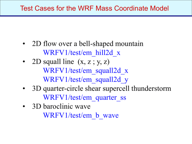
Test Cases for the WRF Mass Coordinate Model
• 2D flow over a bell-shaped mountain
WRFV1/test/em_hill2d_x
• 2D squall line (x, z ; y, z)
WRFV1/test/em_squall2d_x
WRFV1/test/em_squall2d_y
• 3D quarter-circle shear supercell thunderstorm
WRFV1/test/em_quarter_ss
• 3D baroclinic wave
WRFV1/test/em_b_wave
2D Flow Over a Bell-Shaped Mountain
2D Flow Over a Bell-Shaped Mountain
To run: From WRFV1 - compile em_hill2d_x ;
From WRFV1/test/em_hill2d_x –
run ideal.exe, run wrf.exe
Initialization code is in
WRFV1/dyn_em/module_initialize_hill2d_x.F
The terrain profile is set in the initialization code.
The thermodynamic sounding and the initial wind field
is read from the ascii file
WRFV1/test/em_hill2d_x/input_sounding
The 2D solution is computed by integrating the 3D model
with 3 points in periodic direction y; without an initial
perturbation in y the solution remains y-independent.
Setting the terrain heights
In WRFV1/dyn_em/module_initialize_hill2d_x.F
SUBROUTINE init_domain_rk ( grid, &
...
hm = 100.
xa = 5.0
mountain height and half-width
icm = ide/2
mountain position in domain
(central gridpoint in x)
...
Set height
field
DO j=jts,jte
DO i=its,ite ! flat surface
!!
ht(i,j) = 0.
ht(i,j) = hm/(1.+(float(i-icm)/xa)**2)
!
ht(i,j) = hm1*exp(-(( float(i-icm)/xa1)**2))
&
!
*( (cos(pii*float(i-icm)/xal1))**2 )
phb(i,1,j) = g*ht(i,j)
php(i,1,j) = 0.
ph0(i,1,j) = phb(i,1,j)
ENDDO
ENDDO
lower boundary condition
Sounding File Format
File: WRFV1/test/em_quarter_ss/input_sounding
surface
Pressure
(mb)
line 1
each
successive
line is a
point in the
sounding
1000.00
250.00
750.00
1250.00
1750.00
2250.00
2750.00
3250.00
3750.00
4250.00
4750.00
height (m)
surface potential
Temperature (K)
300.00
300.45
301.25
302.47
303.93
305.31
306.81
308.46
310.03
311.74
313.48
potential
temperature (K)
Surface vapor
mixing ratio (g/kg)
14.00
14.00
14.00
13.50
11.10
9.06
7.36
5.95
4.78
3.82
3.01
-7.88
-6.94
-5.17
-2.76
0.01
2.87
5.73
8.58
11.44
14.30
-3.58
-0.89
1.33
2.84
3.47
3.49
3.49
3.49
3.49
3.49
vapor
U (west-east) V (south-north)
mixing
velocity (m/s) velocity (m/s)
ratio (g/kg)
2D squall line simulation
2D squall line simulation
squall2d_x is (x,z), squall2d_y is (y,z); both produce
the same solution.
To run: From WRFV1 - compile em_squall2d_x ;
From WRFV1/test/em_squall2d_x –
run ideal.exe, run wrf.exe
Initialization code is in
WRFV1/dyn_em/module_initialize_squall2d_x.F
This code also introduces the initial perturbation.
The thermodynamic sounding and hodograph
is in the ascii input file
WRFV1/test/em_squall2d_x/input_sounding
3D supercell simulation
Height coordinate model
(dx = dy = 2 km, dz = 500 m, dt = 12 s, 160 x 160 x 20 km domain )
Surface temperature, surface winds and cloud field at 2 hours
3D supercell simulation
To run: From WRFV1 - compile em_quarter_ss ;
From WRFV1/test/em_quarter_ss –
run ideal.exe, run wrf.exe
Initialization code is in
WRFV1/dyn_em/module_initialize_quarter_ss.F
The thermodynamic sounding and hodograph is read
from the ascii input file
WRFV1/test/em_quarter_ss/input_sounding
The initial perturbation (warm bubble) is hardwired
in the initialization code.
Setting the initial perturbation
In WRFV1/dyn_em/module_initialize_quarter_ss.F
SUBROUTINE init_domain_rk ( grid, &
...
!
thermal perturbation to kick off convection
write(6,*) ' nxc, nyc for perturbation ',nxc,nyc
write(6,*) ' delt for perturbation ',delt
DO J = jts, min(jde-1,jte)
yrad = dy*float(j-nyc)/10000.
!
yrad = 0.
DO I = its, min(ide-1,ite)
xrad = dx*float(i-nxc)/10000.
!
xrad = 0.
DO K = 1, kte-1
!
!
!
horizontal radius of the
perturbation is 10 km, centered
at (x,y) gridpoints (nxc, nyc)
put in preturbation theta (bubble) and recalc density. note,
the mass in the column is not changing, so when theta changes,
we recompute density and geopotential
zrad = 0.5*(ph_1(i,k,j)+ph_1(i,k+1,j) &
+phb(i,k,j)+phb(i,k+1,j))/g
zrad = (zrad-1500.)/1500.
RAD=SQRT(xrad*xrad+yrad*yrad+zrad*zrad)
IF(RAD <= 1.) THEN
T_1(i,k,j)=T_1(i,k,j)+delt*COS(.5*PI*RAD)**2
T_2(i,k,j)=T_1(i,k,j)
qvf = 1. + 1.61*moist_1(i,k,j,P_QV)
alt(i,k,j) = (r_d/p1000mb)*(t_1(i,k,j)+t0)*qvf* &
(((p(i,k,j)+pb(i,k,j))/p1000mb)**cvpm)
al(i,k,j) = alt(i,k,j) - alb(i,k,j)
ENDIF
ENDDO
vertical radius of the
perturbation is 1500 m
perturbation added
to initial theta field
maximum amplitude
of the perturbation
Moist Baroclinic Wave Simulation
Height coordinate model (dx = 100 km, dz = 250 m, dt = 600 s)
Surface temperature, surface winds, cloud and rain water
Open Channel Baroclinic Wave Simulation
Day 5
dt = 600 s
dx = dy = 100 km
14000 x 8000 km
Free Slip
Warm Rain
MRF PBL - land
KF Conv. Param.
Ice MIcrophysics
Moist Baroclinic Wave Simulation
To run: From WRFV1 - compile em_b_wave ;
From WRFV1/test/em_b_wave –
run ideal.exe, run wrf.exe
Initialization code is in
WRFV1/dyn_em/module_initialize_b_wave.F
The initial jet (y,z) is read from the binary input file
WRFV1/test/em_b_wave/input_jet
The initial perturbation is hardwired in the
initialization code.
Moist Baroclinic Wave Simulation
Default configuration in
WRFV1/test/em_b_wave/namelist.input
runs the dry jet in a periodic channel with dimension
(4000 x 8000 x 16 km) (x,y,z).
Turning on any microphysics
(mp_physics > 0 in namelist.input) puts moisture
into the basic state.
Switching from periodic to open boundary conditions
along with lengthening the channel produces
a baroclinic wave train.
The initial jet only works for dy = 100 km and
81 grid points in the y (south-north) direction.