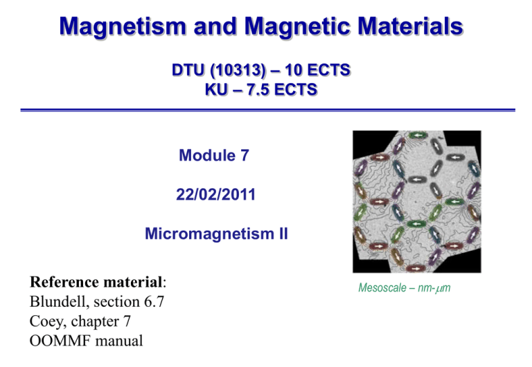
Magnetism and Magnetic Materials
DTU (10313) – 10 ECTS
KU – 7.5 ECTS
Module 7
22/02/2011
Micromagnetism II
Reference material:
Blundell, section 6.7
Coey, chapter 7
OOMMF manual
Mesoscale – nm-mm
Intended Learning Outcomes (ILO)
(for today’s module)
1.
2.
3.
4.
5.
6.
List the various magnetic states found in a rectangular nanoelement after relaxation under no
applied field
Compile a list of energies associated with each magnetic state, and assess whether or not a
correlation exists between energies and statistical expectancy of the states
Simulate Stoner-Wolfharth hysteresis of a single domain rectangular element, and measure
saturation field, remanent magnetization and coercive field
Compare the measurements above with theory and extract an estimate of the demag factors for
the element considered
Create a simple magnetic phase diagram by simulating the magnetic states in circular nanodots
of various geometrical parameters
Compare the numerical phase diagram with theory, and verify that phase boundaries are where
they are expected to be
Flashback
dm2
dm1
Edge effects: the demagnetization field
Domains: flux closure
Dipolar energy and the demag factors
Domain walls: Bloch and Neel
Task 1: Get things running smoothly
13:30-14:00
•Launch OOMMF, and setup a simple problem:
•Square element, 100 nm side, 5 nm thickness, 5 nm cell size.
•Permalloy
•Initialize with random magnetization
•On the mmGraph, choose to display X-iterations, Y1-demag energy, Y2-total energy
•On the mmDisp, choose to display the magnetization, color-coded
•On the mmDataTable, choose to display the total energy
•Let the simulation run until convergence (it should take 5-10 seconds).
•Note what magnetic state you get from this first relaxation
•Now apply a field, and saturate the element along a direction
•Remove the field, and let the system relax
•Do you get the same state as before?
•Discuss within your group, and share your observations with the rest of the class
Task 2: Magnetic states in a rectangular element
14:00-15:00
•Setup the following problem:
•Rectangular element, 300 nm x 200 nm side, 10 nm thickness, 10 nm cell size.
•Permalloy
•Initialize with random magnetization
•On the mmDisp, choose to display the magnetization, color-coded
•On the mmDataTable, choose to display Mx,My,Mz, total energy, exchange energy,
demag energy
•Explore the various states you find on this element by running the simulation many times.
•After each run, note the final value of the total energy from the mmData (which is the
energy of the particular state you end up with)
•How many states did you observe? Take notes, and sketch their appearance on paper.
•Record the frequency of appearance of each of the states. Suppose that, in 100 runs, you get
40 vortices, 20 S-states, etc. Is there a correlation between frequency of appearance of a
state and its energy? One may expect, in fact, that if a state has lower energy, it may be
statistically more likely to appear. But is it really so?
•If you have time, repeat the analysis starting from a uniform magnetization along a
direction different from either the short or the long axis of the element
Task 3: Stoner-Wolfharth hysteresis
15:00-16:00
Task 3 (about 45 min): Stoner-Wolfharth single domain element hysteresis
•Setup the following problem:
•Rectangular element, 200 nm x 100 nm side, 5 nm thickness, 5 nm cell size.
•Permalloy
•Initialize with random magnetization
•On the mmDisp, choose to display the magnetization, color-coded
•On the mmData, choose to display the Mx, My, Mz components, and the energies
•Find the saturation field for the element along a direction 15 degrees off the long axis. Apply a
field, starting from a low value (e.g. a few mT), and increase it in coarse steps until you see the
element saturated along the applied field direction. Take note of the H15_sat, value.
•Setup the field steps to mimic a hysteresis loop: start from H15_sat, decrease to zero and below,
to –H15_sat, in about 20 steps. Relax the element at each field value, and click “Field+” after
you’ve read the Mx value for the next step (we take Mx as a measure of the total magnetization,
although it should be Mx cos(15 degrees)). Repeat until the hysteresis loop completes.
•Observe the evolution of the magnetic state from saturation to reversal. Note in particular what
happens when the applied field happens to reach the value of zero. This is the remanent state. Why
is the value of M at remanence difference from the value of M at saturation?
Task 4: A simple magnetic phase diagram
16:00-17:00
•Consider a single domain magnetic dot (a cylinder of some radius R and height t). There are three
competing states: in-plane magnetization, axial magnetization, and vortex state. Which one is the
lowest energy, depending on the choice of R and t? If the dot is very very thick, you may expect it
to be magnetized axially. If the dot is very thin, you may expect it to be magnetized in-plane. If it’s
somewhere in between, perhaps the vortex state will appear. Where exactly are the phase
boundaries? I.e. the boundaries in parameter space separating ground states?
•Choose a setup that allows you to explore the energy landscape of magnetic dots, and create a
magnetic phase diagram, where on the x-axis you put the radius, on the y-axis you put the height.
Run several simulations, and assign a “V” in the (R,t) location where you found a vortex, a “X”
where you found an in-plane state, and a “A” in case you got an axial magnetization.
•When you get vortices, please have a look at what happens to the vortex core, i.e. the center of the
vortex. What do you notice? And why?
•Think of what may happen if a small applied field is applied to a circular dot in the vortex state.
Write down your prediction, and then try a simulation to verify if you were correct.
Wrapping up and sneak peek
•Micromagnetic simulations with OOMMF
•Variety of relaxed states
•Stoner-Wolfharth hysteresis
•Coercive and saturation fields, remanent magnetization
•Magnetic phase diagrams
•The vortex core in circular nanodots
Next lecture: Friday February 25, 8:15, KU (411D)
Permanent magnets (MB)