151 Project 3
Bison Management
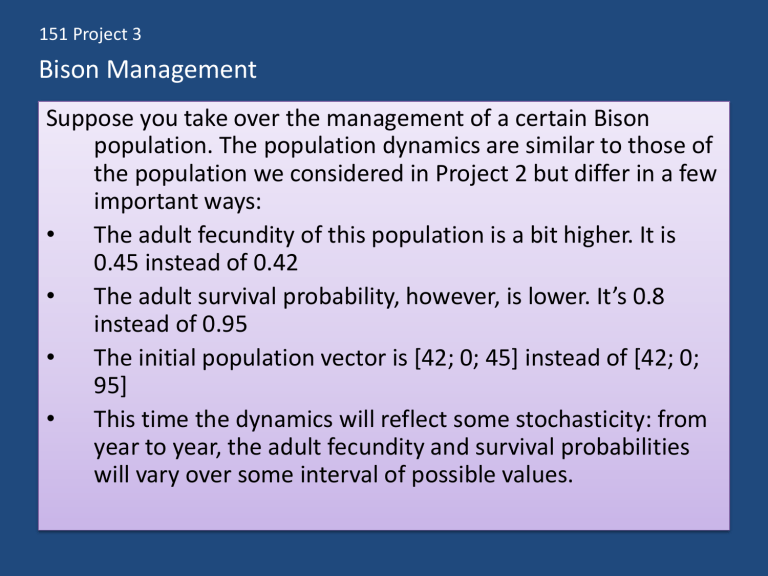
Suppose you take over the management of a certain Bison population. The population dynamics are similar to those of the population we considered in Project 2 but differ in a few important ways:
• The adult fecundity of this population is a bit higher. It is
0.45 instead of 0.42
• The adult survival probability, however, is lower. It’s 0.8 instead of 0.95
• The initial population vector is [42; 0; 45] instead of [42; 0;
95]
• This time the dynamics will reflect some stochasticity: from year to year, the adult fecundity and survival probabilities will vary over some interval of possible values.

151 Project 3
Bison Management
First off, let’s re-open our m-file for Project 2, question 1.a:

151 Project 3
Bison Management
Now update the fecundity & survival rates, and initial condition:

151 Project 3
Bison Management
Before adding the randomness, let’s run the model:
Population seems to be growing.

151 Project 3
Bison Management
Let’s modify our m-file for question 1.b. to see a graph:
Again, seems to be growing. How can we know for sure?

151 Project 3
Bison Management
We find the dominant eigenvalue! If it’s greater than 1, then the population will grow:
It is greater than 1, but notice that it is not much greater. This should indicate to us that small changes could be bad news for our bison.

151 Project 3
Bison Management
Now we need to add some randomness.
• Suppose that shortly after we took on this management job, we learned that the population is doing about as good as we could hope; that is, the current parameter values are historically high.
• From our perspective we decide to be conservative and assume that it will never be better that it is now.
• We determine from data that the adult survival probability ranges from 0.77 to 0.80 from year to year.
• Before adding randomness for adult fecundity, let’s explore the case where only survival probability varies.

151 Project 3
Bison Management
Make the following changes to your code:

151 Project 3
Bison Management
Remarks about the changes we just made:
1.
Notice that the adult survival rate (the (3,3) entry of matrix
A) is being changed each year. Let’s look at the MATLAB command “rand”:
The command rand(1) always returns a random number between 0 and 1.

151 Project 3
Bison Management
We want to use this MATLAB function to choose a random number on an interval of our choosing- in this case, the interval (0.77,0.80). The command, “0.8-.03*rand(1)” accomplishes this:
This explains the line of code that updates our matrix each time step.

151 Project 3
Bison Management
(continued) Remarks about the changes we just made:
2.
Recall that we were able to derive a formula to give us the population at time t without needing to calculate the population values for all the previous time steps:
  
A

v t

v t

A t  v
 
This formula allows to find the population size at the
next time step.
This formula allows to find the population size at any time step.

Notice that one of the changes we just made was swapping out the formula shown here on the right-hand side for the one on the left-hand side. Why would we want to do this?

151 Project 3
Bison Management
Answer: We want to change the matrix A every time step
(explained in remark 1) and we want to “remember” all of the previous information. The other formula would indeed reflect the change made to the matrix every time step but it would “erase” the previous changes by “going back”, as it were, and using this new matrix to recalculate all of the past values for v. You should think about why this is the case.
3. Finally, since we are only going to concern ourselves with the question of extinction, we get rid of the table showing the population values from year to year. We need only inspect the population size at the end of our simulation. The population size at the end of the simulation will be determined by looking at the vector v.

151 Project 3
Bison Management
At the end of the 200 year run, the vector v will contain the population size of calves, yearlings, and adults at time step
200. To check for extinction, we observe the following:
– We need to round the components of this vector so that it makes sense for a population. That is, it doesn’t make sense to say we have
3.9462 calves. We could reasonably say 4 calves. This explains why we use the command, “round(v)”
– To check for extinction it is sufficient to add the 3 elements of vector v and check if they sum to zero. This explains why we use the command, “sum(round(v))”
– To see this, run the code and This is the final time, rounded population vector.
you will get output like this:
This is the sum of the entries of that vector.

151 Project 3
Bison Management
Next, make the following changes to your code:

151 Project 3
Bison Management
Remarks about the changes we just made:
1.
We already had one for-loop that forecasted our population out to 200 time steps. Now we’d like to simulate this process, say, 1000 times. So we need to encase our existing loop within another loop. This explains the line of code, “for i=1:1000” and the “end” to which it is attached.
2.
After each 200 year run, we need to see if the population is extinct. That is why we ask, “if sum(round(v))==0”. MATLAB will check to see if this condition is true. (When checking for an equality- as we are here- we have to use two equal signs.) If the condition is true, then MATLAB will carry out the following command. Otherwise, it will do nothing and move past the “if-end” line of code.

151 Project 3
Bison Management
(continued) Remarks about the changes we just made:
3. Now, if the population is extinct, we need to somehow take note of this fact. An easy way to accomplish this is to simply count how many times it happens. We start off with the count equal to zero.
This explains the very first line of code where we initialize our extinction count, E, to be zero.
4.
Then the first time our population goes extinct, MATLAB will set
E=E+1 which would be E=0+1=1. The next time our population goes extinct, MATLAB will set E=E+1 which would be E=1+1=2.
And so on. This explains the other part of the “if-end” line of code.
5.
Finally, after the 1000 simulations, we ask MATLAB to output the percentage of the simulations wherein the population went extinct. This explains the very last line of code, “E/1000”

151 Project 3
Bison Management
Now, let’s run this code a few times. Here’s the output from the command window:
I ran the 1000 simulations of a 200 year forecast, 4 times. The population never went extinct!

151 Project 3
Bison Management
Now, let’s fix S back to 0.8 and repeat the previous steps with F ranging over (0.31, 0.45):
Notice that instead of deleting the line of code for varying S,
I have simply put a % in front of it. Now MATLAB won’t execute that line. This is handy since I want to use that line later. I won’t have to retype it; I just delete the %.

151 Project 3
Bison Management
Now, let’s run this code a few times. Here’s the output from the command window:
I ran the 1000 simulations of a 200 year forecast, 5 times. The population went extinct approximately 13% of the time.

151 Project 3
Bison Management
Summary so far:
• When we let S vary over the interval (0.77, 0.80), our population never went extinct.
• When we let F vary over the interval (0.31, 0.45), our population went extinct ~13% of the time.
Your tasks from here:
1) Without running the code, predict what will happen if you let both parameters vary. Now run the code and compare the results with your prediction.
2) Suppose you’ve been given a budget for management of the population.
You can afford to either: a) Raise the lower bound of F by 0.05 to get (0.36,0.45) b) Raise the lower bound of S by 0.027 to get (0.797,0.80)
Based on the first 3 questions, predict which strategy you think is best. Explain your reasoning.
3) Now run the code several times for each strategy. Write down the results for each strategy. Which one should you choose? How does this compare with your prediction?