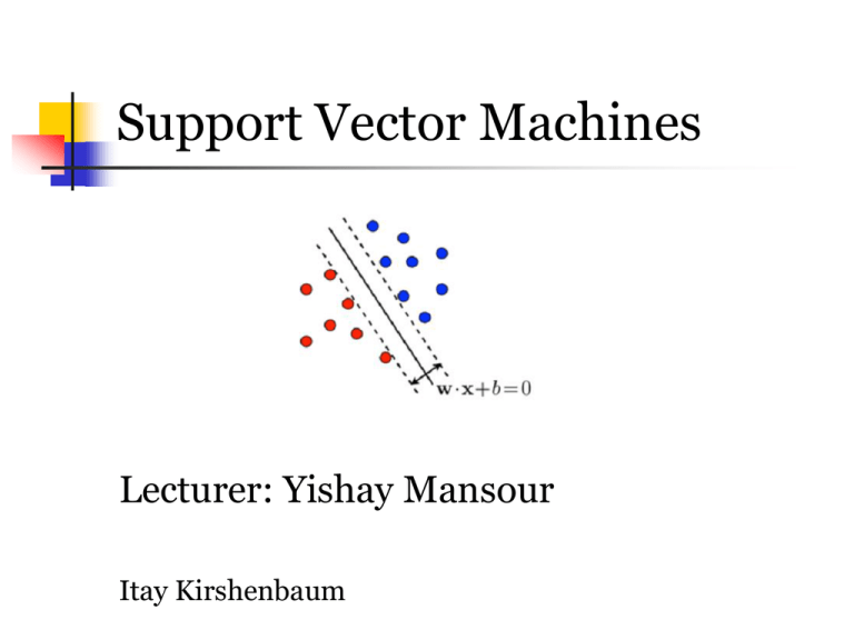
Support Vector Machines
Lecturer: Yishay Mansour
Itay Kirshenbaum
Lecture Overview
In this lecture we present in detail one of
the most theoretically well motivated and
practically most effective classification
algorithms in modern machine learning:
Support Vector Machines (SVMs).
Lecture Overview – Cont.



We begin with building the intuition
behind SVMs
continue to define SVM as an
optimization problem and discuss how
to efficiently solve it.
We conclude with an analysis of the
error rate of SVMs using two
techniques: Leave One Out and VCdimension.
Introduction



Support Vector Machine is a supervised
learning algorithm
Used to learn a hyperplane that can
solve the binary classification problem
Among the most extensively studied
problems in machine learning.
Binary Classification Problem





Input space: X  R
Output space: Y  {  1,  1}
Training data: S  {( x1 , y 1 ),..., ( x m , y m )}
S drawn i.i.d with distribution D
Goal: Select hypothesis h  H that best
predicts other points drawn i.i.d from D
n
Binary Classification – Cont.

Consider the problem of predicting the
success of a new drug based on a patient
height and weight




m ill people are selected and treated
This generates m 2d vectors (height and
weight)
Each point is assigned +1 to indicate
successful treatment or -1 otherwise
This can be used as training data
Binary classification – Cont.



Infinitely many ways to classify
Occam’s razor – simple classification
rules provide better results

Linear classifier or hyperplane

h  H maps x  X to  1 if ( w * x  b )  0
Our class of linear classifiers:
H  {x  sign ( w * x  b ) | w  R , b  R }
n
Choosing a Good Hyperplane

Intuition

Consider two cases of positive
classification:




w*x + b = 0.1
w*x + b = 100
More confident in the decision made by the
latter rather than the former
Choose a hyperplane with maximal
margin
Good Hyperplane – Cont.

Definition: Functional margin S
ˆ s 
min
i
i
i
i
ˆ with ˆ  y ( w * x  b )
i{1 ,..., m }
i
i
y is the classifica tion of x according to ( w , b )

A linear classifier:
Maximal Margin

w,b can be scaled to increase margin



sign(w*x + b) = sign(5w*x + 5b) for all x
(5w, 5b) is 5 times greater than (w,b)
Cope by adding an additional
constraint:

||w|| = 1
Maximal Margin – Cont.

Geometric Margin

Consider the geometric distance between
the hyperplane and the closest points
Geometric Margin

Definition: Geometric margin S
s 
min
 with 
i
i
 y (
i
w
i{1 ,..., m }

*x 
i
b
w
Relation to functional margin
ˆ  w  y
i

w
i
Both are equal when
w 1
)
The Algorithm

We saw:




Two definitions of the margin
Intuition behind seeking a maximizing
hyperplane
Goal: Write an optimization program
that finds such a hyperplan
We always look for (w,b) maximizing
the margin
The Algorithm – Take 1

First try:
max   y ( w * x  b )   , i  1,..., m , w  1
i

Idea



i
Maximize  - For each sample the
Functional margin is at least 
Functional and geometric margin are the
same as w  1
Largest possible geometric margin with
respect to the training set
The Algorithm – Take 2

The first try can’t be solved by any offthe-shelf optimization software



The w  1 constraint is non-linear
In fact, it’s even non-convex
How can we discard the constraint?

Use geometric margin!
max
ˆ
w
i
i
 y ( w * x  b )  ˆ , i  1,..., m
The Algorithm – Take 3


We now have a non-convex objective
function – The problem remains
Remember





We can scale (w,b) as we wish
Force the functional margin to be 1
1
Objective function: max
w
1
Same as: min w
2
Factor of 0.5 and power of 2 do not change
the program – Make things easier
2
The algorithm – Final version

The final program:
max
1
2



w
2
 y ( w * x  b )  1, i  1,..., m
i
i
The objective is convex (quadratic)
All constraints are linear
Can solve efficiently using standard
quadratic programing (QP) software
Convex Optimization


We want to solve the optimization
problem more efficiently than generic
QP
Solution – Use convex optimization
techniques
Convex Optimization – Cont.

Definition: A convex function
f
 x , y  X ,   0 ,1 :
f (  x  (1   ) y )   f ( x )  (1   ) f ( y )

Theorem
Let f : x   be a differenti able convex function
 x , y  X : f ( y )  f ( x )   f ( x )( y  x )
Convex Optimization Problem

Convex optimization problem
Let f , g i :x   , i  1,.., m be convex function
Find min

x X
f ( x ) s.t. g i ( x )  0 , i  1,.., m
We look for



a value of x  X
Minimizes f ( x )
Under the constraint
g i ( x )  0 , i  1,.., m
Lagrange Multipliers



Used to find a maxima or a minima of a
function subject to constraints
Use to solve out optimization problem
Definition
Lagragian
L of function
f subject to constraint s
g i , i  1,.., m
m
L ( x, )  f ( x) 

i
g i ( x) x  X , i  0
i 1
 i are called the Lagrange Multiplier s
Primal Program

Plan




Use the Lagrangian to write a program
called the Primal Program
Equal to f(x) is all the constraints are met
Otherwise – 
Definition – Primal Program
 P ( x )  max
 0
L ( x, )
Primal Progam – Cont.


The constraints are of the form
If they are met  P ( x )  f ( x )
m

is maximized when all
 i are 0, and the summation is 0

i
gi ( x)
i 1

Otherwise  P ( x )  
m


i 1
i
gi ( x)
is maximized for  i
 
gi ( x)  0
Primal Progam – Cont.

Our convex optimization problem is
now:
min

x X
 P ( x )  min
x X
max
 0
L ( x, )
 P ( x ) as the value of
Define
x X
the primal program
p  min
*
Dual Program

We define the Dual Program as:
 D ( x )  min

L ( x, )
We’ll look at
max



x X
a0
min
x X
 D ( x )  max
a0
min
x X
L ( x, )
Same as our primal program
Order of min / max is different
Define the value of our Dual Program
d  max
*
a0
min
x X
L ( x, )
Dual Program – Cont.

We want to show


*
*
If we find a solution to one problem, we
find the solution to the second problem
Start with d *  p *

“max min” is always less then “min max”
d  max
*

d  p
a0
min
x X
L ( x ,  )  min
Now on to p *  d *
x X
max
a0
L ( x, )  p
*
Dual Program – Cont.

Claim
if exists x and a  0 which are a saddle point and
*
*
 a  0 ,  x which is feasible : L ( x , a )  L ( x , a )  L ( x , a )
*
*
then p  d and x is a solution t o  p ( x )
*

*
*
Proof
p  inf sup L ( x , a )  sup L ( x , a )  L ( x , a )
*
*
x
a0
a0
 inf L ( x , a )  sup inf L ( x , a )  d
*
x

*
Conclude
x
a0
d  p
*
*
*
*
*
*
Karush-Kuhn-Tucker (KKT)
conditions


KKT conditions derive a
characterization of an optimal solution
to a convex problem.
Theorem
Assume that f and g i , i  1,.., m are differenti able and convex.
x is a solution t o the optimizati on problem     0 s.t. :
1.  x L ( x ,  )   x f ( x )     x g ( x )  0
2.  a L ( x , )  g ( x )  0
3.  g ( x ) 

i
gi(x)  0
KKT Conditions – Cont.

Proof
For every feasible x :
f ( x)  f ( x )   x f ( x )  ( x  x )
 
 
 

m
i 1
m
i 1
m
i 1
ai x g i ( x )  ( x  x )
a i [ g i ( x )  g i ( x )]
ai g i ( x)  0
The other direction holds as well
KKT Conditions – Cont.

Example

Consider the following optimization
1
problem: min x s .t . x  2
2 1
We have f ( x )  x , g ( x )  2  x
2
1
L
(
x
,

)

x   (2  x)
The Lagragian will be
2


2
1
2
L
x
2
 x   0  x  
*
*
L( x , ) 
*
1
2


   ( 2   )  2 
2
1

2
L( x , )  2    0    2  x
*
*
2
Optimal Margin Classifier

Back to SVM

Rewrite our optimization program
min
1
w
2
 y ( w * x  b )  1, i  1,..., m
i
i
2
g i (w, b)   y (w * x  b)  1  0
i

Following the KKT conditions


i
i  0
Only for points in the training set with a
margin of exactly 1
These are the support vectors of the
training set
Optimal Margin – Cont.
Optimal margin classifier and its
support vectors

Optimal Margin – Cont.

Construct the Lagragian
L (w, b, ) 
1
w
m
2

2


[ y ( w * x  b )  1]
i
i
i
i 1
Find the dual form


First minimize L ( w , b ,  ) to get 
Do so by setting the derivatives to zero
D
m
 x L (w, b, )  w 

i 1
m
 w 
*

i 1
i
i
y x
i
iy x  0
i
i
Optimal Margin – Cont.

Take the derivative with respect to

b

m
L (w, b, ) 

iy  0
i
i 1
Use w * in the Lagrangian
m
L(w , b , ) 
*
*
 i 
i 1

b
1
m

m
y y  i j x x  b   i y
i
2 i , j 1
j
i
j
i 1
We saw the last tem is zero
m
L(w , b , ) 
*
*
 i 
i 1
1
m

2
i , j 1
y y  i j x x
i
j
i
j
 W ( )
i
Optimal Margin – Cont.

The dual optimization problem
max W ( ) :  i  0 , i  1,.., m
m

y  0
i
i
i 1

The KKT conditions hold

*
Can solve by finding  that maximize W ( )
Assuming we have – define w    y x
The solution to the primal problem
m

*
*
i 1

i
i
Optimal Margin – Cont.

Still need to find


Assume
We get
x
i
b
is a support vector
1  y (w  x  b )
i
*
i
*
y  w x b
*
b  y w x
i
i
*
*
i
*
i
*
Error Analysis Using LeaveOne-Out

The Leave-One-Out (LOO) method




Remove one point at a time from the
training set
Calculate an SVM for the remaining points
Test our result using the removed point
Definition

1
m
I (h
(x )  y )

m
The indicator function I(exp) is 1 if exp is
true, otherwise 0
Rˆ LOO 
i
i
i 1
S { x }
i
LOO Error Analysis – Cont.

Expected error
E S ~ D m [ Rˆ LOO ] 
1
m
m

i 1
E [ I ( h S  { x i } ( x )  y )] 
i
i
E S , X [ h S  { x i } ( x )  y ]  E S ' ~ D m 1 [ error ( h S ' )]
i

i
It follows the expected error of LOO for a
training set of size m is the same as for a
training set of size m-1
LOO Error Analysis – Cont.

Theorem
E S ~ D m [ error ( h S )]  E S ~ D m 1 [
N SV ( S )
m 1
]
N SV ( S ) is the number of support ve ctors in S

Proof
if h S classifies a point incorrectl y, the point must be a support ve ctor.
N SV ( S )
ˆ
Hence : R LOO 
m 1
Generalization Bounds Using
VC-dimension

Theorem
Let S  x : x  R . Let d be the VC - dimension
set sign ( w  x ): min

Proof
x S

w  x   , w   . Then d 
1
Assume that the set x ,.., x
d
 is shattered.
d  w  y x  w 
i
i 1
i
d

i 1
d
i
y x
i


i 1
i
y x
2

2
2
i
i
d
R 
So for every y   1,  1
 w :   y ( w  x ) i  1,.., d . Summing over d :
i
of the hyperplane
i
Generalization Bounds Using
VC-dimension – Cont.

Proof – Cont.
Averaging over the y ' s with uniform distributi on :
1
d
d  E y

i
y x
 E 2 y
i
i 1
2
d

i
y x
E y [ x x y y ]

i
i
i 1
j
i
j
i, j
Since E y [ y y ]  0 when i  j and E y [ y y ]  1 when i  j
i
j
i
j
we can conclude that :
 d   E y [ x x y y ]  
i
j
i, j
j

i
R 
2
Therefore d 
i

2
2
2
x
i
  dR
2