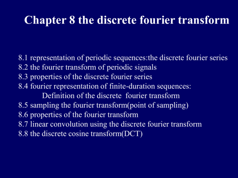
Chapter 8 the discrete fourier transform
8.1 representation of periodic sequences:the discrete fourier series
8.2 the fourier transform of periodic signals
8.3 properties of the discrete fourier series
8.4 fourier representation of finite-duration sequences:
Definition of the discrete fourier transform
8.5 sampling the fourier transform(point of sampling)
8.6 properties of the fourier transform
8.7 linear convolution using the discrete fourier transform
8.8 the discrete cosine transform(DCT)
8.1 representation of periodic sequences:
the discrete fourier series
1
~
x[ n] 


N

~
 X [k ] 


kn
WN
e
N 1

~
 kn
X [ k ]WN
(1), n  0,..N  1
k 0
N 1 ~
 x[n]WN (2), k  0,..N  1
kn
n 0
 j 2kn / N
~
X [ k  rN ] 
( k  rN ) n ~
~
X [k ]
 x [n]W
N
n 0
N 1
EXAMPLE.
Figure 8.1
~
X [k ] 
4

n 0
kn
W10
e
N=10
 j 4k / 10
sin(k / 2)
sin(k / 10 )
phase X denotes：magnitude=0，phase is indeterminate
Figure 8.2
8.2 the fourier transform of periodic signals
2
~
N 1
2 ~
2k
~ j
 X [k ]
X (e )  
X [k ] ( 
)
N
N
N
k 0

0


2
N
other
dispersion in time domain results in periodicity in frequency domain;
Periodicity in time domain results in dispersion in frequency domain.
DFS is a method to calculate frequency spectrum of periodic signals.
k
FIGURE 8.5
8.3 properties of the discrete fourier series
DFS ~
DFS ~
DFS ~
~
~
~
x [ n]
X [k ], x1[n]
X 1[k ], x2 [n]
X 2 [k ]



DFS ~
~
~
~
1.linearity : ax1[n]  bx2 [n]
aX 1[k ]  bX 2 [k ]

N=4，12 points DFS
two periodic
sequences with
different period
N=6，12 points DFS
both period=12
compositive sequence N=12，12 points DFS
2.shift of
DFS km ~
~
a sequence : x [n  m]
W
X [k ]

N
nl ~
DFS ~
W
x [ n]
X [k  l ]
N

DFS ~
~
3.duality : X [n]
Nx [k ]

4.symmetry properties:
DFS ~
DFS ~
~
~
x * [n]
X * [k], x * [n]
X * [k]


DFS 1 ~
1 ~
~
~
~
~
Re{ x[n]}  (x[n]  x * [n])
(X[k]  X * [k])  X e [k]
 2
2
DFS 1 ~
1 ~
~
~
~
~
jIm{ x[n]}  (x[n]  x * [n])
(X[k]  X *[k])  X o [k]
 2
2
DFS 1 ~
1 ~
~
~
~
~
x e [n]  (x[n]  x *[n])
(X[k]  X *[k])  Re{ X[k ]}
 2
2
DFS 1 ~
1 ~
~
~
~
~
xo [n]  ( x [n]  x * [n])
( X [k ]  X * [k ])  j Im{ X [k ]}
 2
2
For a real sequence:
~
~
x[n]  x*[n]
~
~
X [k ]  X *[k ]
~
~
Re{ X [ k ]}  Re{ X [  k ]}
~
~
Im{ X [ k ]}   Im{ X [  k ]}
~
~
| X [ k ] || X [  k ] |
~
~
 X [k ]    X [k ]
EXAMPLE.
DFS of real sequence
FIGURE 8.2
5. periodic convolution :
N 1
~
x3 [n]  ~
x1[n]  ~
x2 [ n ]   ~
x1[m]~
x2 [ n  m ]  ~
x2 [ n ]  ~
x1[n]
m 0
Periods of 3 sequences are all N.
(1)if : ~
x3 [n]  ~
x1[n]  ~
x2 [n]
~
~
~
then : X 3 [k ]  X 1[k ] X 2 [k ]
(2)if : ~
x3 [n]  ~
x1[n]~
x2 [n]
~
~
then : X 3 [k ] 
1
N
~
X [k ]  X 2 [k ]
1
graphic method to
calculate periodic
convolution
Figure 8.3
8.4 fourier representation of finite-duration sequences:
Definition of the discrete fourier transform
~
x [ n] 

 x[n  rN ]  x[n mod N ]  x[(( n)) N ]
r  
~
x[n]  x[n]RN [n]
EXAMPLE.
Figure 8.8
The last two expressions are
only suitable to no aliasing.
Two derivations of definition:
1. Periodic extension of the finite-duration sequence with
period N ;
DFS of the periodic sequence ;
DFT is the dominant period of DFS.
2. DTFT of the finite-duration sequence;
DFT is the N-points spectral sampling.
duration of sequence is N
N 1

kn
 X [k ] 
x[ n]WN , k  0,1,....N  1


n 0

N 1
1

 kn
x
[
n
]

X
[
k
]
W
, n  0,1,...N
N

N

k 0



N 1

X [0]   x[ n]


n 0

1 N 1
 x[0] 
X [k ]


N k 0

X [ k ]  X (e
j
)|

2
N
 X ( z) |
k
z e
j
2
N
k
EXAMPLE.
Figure 8.10
periodic
extension
with period 5
x[(( n)) 5 ]
DFS{~
x [n]}
~
X [ k ]R5 [ k ]
explanations：1. DFT and DFS have the same expression, but
DFT are samples of frequency spectrum of the finite-duration
sequence , DFS is frequency spectrum of periodic sequence。
2. the periods of DFS in time and frequency domain is N,
DFT in frequency domain is defined to be finite duration, but
has the immanent period N。
3. the meaning of DFT not only is samples of frequency
spectrum , but also can reconstruct time-domain signal。
8.5 sampling the fourier transform
EXAMPLE.
Figure 8.5
periodic
extension with
period 10
reflect
frequency
spectrum of
signal more
truly than
figure 8.10
conclusion ：sequence with length N is extended to M by filling 0
in time domain, then do M-points DFT. We can get more dense
samples of its FT, and can reconstruct time-domain signal by
taking the first N nonzero values from the reconstructed signal。
contrarily, if we want to get M-points samples of FT by DFT,
we can use the method of filling 0 in time domain.
genetic instance：
Sequence with length N（or infinite length）, sample M points in
frequency domain（more than or less than or equal to N），then
the reconstructed time-domain signal is dominant period of the
periodic extension with period M of original signal（maybe

aliasing）。Viz. if
X (e
j
)|

2

k
M
then the result of IDFT is ：

kn
x[ n]WM , k  0,1...M  1
n  

x'[n]  (  x[ n  rM ]) RN [n]
r  
Conclusion：when M<N, the reconstructed time-domain signal is
domain period of the periodic extension with aliasing of original
signal. Contrarily , if we want to get M (M<N) sample points of FT
by DFT，we can extend the sequence with period M in time
domain, take the dominant period and do M-points DFT.
sampling theorem in frequency domain：
If sampling points N in frequency domain is more than the length
of sequence ，the time-domain signal can be reconstructed；
and the sampling spectral line can be constructed to be
continuous spectral function by ideal interpolation：
X (e

j
)  1 e
 jN
N 1
/ N 
X [k ]
k
k  0 1  WN e
 j
prove :
X (e
j
N 1
)   x[ n]e
 j n
n 0

1
N
N 1
N 1
N 1
 (
n 0
 X [k ](WN e
k 0
 1  e
 jN
 kn
 jn
1
N
)
n 0
N 1
/ N 
k 0
X [k ]
k
1  WN e
 j
N 1
 X [k ]WN
k 0
 kn
)e
 j n
DFT of a finite-duration sequence、DFS of a periodic sequence are
both samples of FT of another sequence, then the relationship
among the three sequences in time domain：
M points IDFT
X [k ]
2
M点取样
FT
x1[n]  X1 (e
j

 

x2 [n]    x[n  rM ]  RM [n]
 r  

取长为M
的主周期
)
M点IDFS
~
~
M点取样 X 3[k ]  x3[n] 

 x[n  rM ]
r  
periodic extension in time domainsampling in frequency domain
summary 8.5
1. DFT is N-points samples of frequency spectrum of sequence with length N. the
more spectral sampling points, the more genuine to reflect the frequency spectrum
2. get M-points spectral samples of N-points sequence by M-points DFT:
（1）M=N，do M-points DFT directly
（2）M>N，extend x[n] to M points by filling 0，then do M-points DFT
（3）M<N，periodic extension of x[n] with period M and aliasing ，take the
dominant period with length M, then do M-points DFT
3. whether spectral sampling can reconstruct original time-domain signal
spectral sampling theorem ：if spectral sampling points is larger than or equal
to the length of signal, the time-domain signal can be reconstructed. Contrarily, it
can not be done.
4. If frequency spectrum is the same，its samples are equal；contrarily, it does
not come into existence。
if frequency spectrum has linear phase, its samples has linear phase, too；
contrarily, it does not come into existence 。
8.6 properties of the fourier transform
x[n]
DFT

X [k ], x1[n]
DFT

1.linearity : ax1[n]  bx2 [n]
X 1[k ], x2 [n]
DFT

DFT

aX1[k ]  bX 2 [k ]
2.circular shift of a sequence
x1[n]  x[(( n  m)) N ]RN [n]  x[(( n  ( N  m))) N ]RN [n]
x[((n  m)) N ]RN [n]
W
 ln
N
x[n]
DFT

DFT

W
km
X [k ]
N
X [((k  l )) N ]RN [k ]
X 2 [k ]
EXAMPLE.
circular
shift
Figure 8.12
EXAMPLE. （8.42）
| H1[k ] |
8points DFT| H [k ] |
2
h1[n]
h2 [n]
| H1 (e
j
) | 1024 points DFT
| H 2 (e
j
)|
3.duality : X [n]
DFT

Nx[((k )) N ]RN [k ]  Nx[ N  k ]
EXAMPLE.
x[n]  n cos(0.2n)
| X [k ] || DFT {x[n]} |
DFT { X [n]}
X '[k ]  X [(( k )) N ]RN [k ]  X [(( N  k )) N ]RN [k ]  X [ N  k ]
X [k ]
X '[k ]
4. Symmetry properties:
*
x [ n]
DFT

*
*
*
X [((k )) N ]RN [k ]  X [(( N  k )) N ]RN [k ]  X [ N  k ]
*
*
x [((n)) N ]RN [n]  x [ N  n]
Re{ x[n]} 
1
( x[n]  x * [n])
DFT

DFT 1
*
X [k ]
( X [k ]  X * [ N  k ])  X ep [k ]
 2
2
DFT 1
1 ~
~
~
j Im{x [n]}  ( x [n]  x * [n])
( X [k ]  X * [ N  k ])  X op[k ]
 2
2
xep [n] 
1
xop[n] 
1
( x[n]  x * [ N  n])
DFT 1
2
2
( x[n]  x * [ N  n])
( X [k ]  X * [k ])  Re{ X [k ]}
 2
DFT 1
 2
( X [k ]  X * [k ])  j Im{ X [k ]}
definition ：
X ep [ k ] : periodic conjugate - symmetric components
X op [ k ] : periodic conjugate - antisymmet ric components
sequence with length N can be decomposed ：
X [ k ]  X ep [ k ]  X op [ k ]
while ：
X ep [ k ] 
1
2
( X [ k ]  X * [ N  k ])  X ep * [ N  k ]，length N
real part is even symmetric , imaginary part is odd symmetric
X op [ k ] 
1
2
( X [ k ]  X * [ N  k ])   X op * [ N  k ]，lenth N
real part is odd symmetric , imaginary part is even symmetric
For a real sequence:
x[n]  x * [n]
X [k ]  X * [ N  k ]
Re{ X [k ]}  Re{ X [ N  k ]}
Im{ X [k ]}   Im{ X [ N  k ]}
| X [k ] || X [ N  k ] |
 X [k ]    X [ N  k ]
EXAMPLE. x[n]  0.5n  cos(0.5n), n  0...9
Real{X[k]}
|X[k]|
N=10
DFT of real
sequence
Imag{X[k]}
arg{X[k]}
N=9
|X[k]|
Arg{X[k]}
5.circular convolution
y[n]  x1[n]( N ) x2[n]
 ( x1[((n)) N ]  x2[((n)) N ])RN [n]
N 1
(
 x [((m))
1
N ] x2 [((n  m)) N ]) RN [ n]
m 0
Length of x1[n],x2[n],y[n] are N.
(1) x1[n]( N ) x2 [n]
(2) x1[n]x2 [n]
DFT

DFT 1
 N
X 1[ k ] X 2 [ k ]
X 1[k ]( N ) X 2 [k ]
EXAMPLE.
graphic
method to
calculate
circular
convolution
x[n]( N ) [n  1]
 x[(( n  1)) N ]RN [n]
Figure 8.14
convolution
result
depends on
N
EXAMPLE.
Figure 8.15
N=L
Figure 8.16 N=2L
EXAMPLE.
6.paswal’s theory
N 1
N 1
 x[n] y * [n]  N  X [k ]Y * [k ]
1
n 0
k 0
N 1

n 0
2
| x[ n] | 
1
N
N 1

k 0
2
| X [k ] |
8.7 linear convolution using the discrete fourier
transform
if : y[n]  x[n] * h[n]

then : x[n（
] N）h[n] 
 y[n  rN ]R
N [ n]
r  
PROVE
x[n]  h[n]

y[n]
FT
X (e
j
) H (e
j
)

Y (e
j
)
N point sample
according
to
properties
of circular
convolution
X [k ]H [k ]

IDFT
x[n]( N )h[n]

Y [k ]
according
to spectral
sampling

 y[n  rN ]R
r  
If N>=N1+N2-1,then x[n]*h[n]=x[n](N)h[n]
N [ n]
EXAMPLE.
Figure 8.18
linear convolution
shift right of the
linear convolution
shift right of the
linear convolution
6 points circular convolution=
linear convolution with
aliasing
12 points circular convolution
= linear convolution
Conclusion:
(1)calculate N point circular convolution by linear convolution
(a) y[n]  x[n] * h[n]

(b) x[ n]( N )h[n] 
 y[n  rN ]R
N [ n]
r  
(2) calculate linear convolution by circular convolution
(a) zero  padding x[n] and h[n] to length of N  L1  L2  1
(b) x[n]  h[n]  x[n]( N )h[n]
(3) calculate linear convolution by DFT
(a) zero  padding x[n] and h[n] to length of
(b) N po int s DFT of
x[n] and h[n]
(c) x[n]( N )h[n]  IDFT { X [k ]H [k ]}
x[n] * h[n]  x[n]( N )h[n]
N  L1  L2  1
implementing linear time-invariant FIR systems using the DFT
Figure 8.22
consideration：
（1）deal with data when input them
（2）operation speed
（3）the counts of input and output data are equal
the following two methods is used
in the situation such that real-time
and speedy operation is required；
time-domain method is commonly
used。
overlap-add method
length of h[n] is P
(1)segment x(n) into sections of length L;
(2)fill 0 into h(n) and some section of x(n) ,
then do L+P-1 points FFT ;
(3) calculate
y (n)  IFFT {H (k ) X (k )}，n  0,...L  P  2
(4)add the points n=0…P-2 in y (n) to the
last P-1 points in the former section y[n]，
the output for this section is the points
n=0…L-1
y0 (n)  0  h[0]  0  h[1]  0  h[2]  x[n  3]h[3]  ...
n  L,...L  P  2
y1 (n)  x[n]  h[0]  x[n  1]  h[1]  x[n  2]  h[2]
 0  h[3]  0  h[4]  ..., n  0,..P  2
y2 (n)  y1[n]  y2 [n], n  0,...P  2
P-1 points
overlap-save method
the length of h[n] is P
(1)segment x(n) into sections of length L,
overlap P-1 points;
(2)fill 0 into h(n) and some section of x(n) ,
then do L points FFT ;
(3) calculate
y(n)  IFFT{H (k ) X (k )}，n  0,...L  1
(4) the output for this section is the L-P+1
points n=P-1,…L-1 of y[n]
If do L+P-1 points DFT, then wipe off the
first and last P-1 points in the result,
respectively, output is the middle L-P+1
points。
To guarantee the output is linear convolution
result, the minimum points of DFT is L。
Figure 8.24
P-1 points
linear convolution
result
Conclusion : use of DFT：
（1）calculate spectral sample of signals
（2）calculate sample of frequency response of systems
（3）frequency-domain realization for FIR system
8.8 the discrete cosine transform(DCT)
DCT  1：X [ k ] 
x[ n] 
DCT  2：X [ k ] 
N 1
ck
2
N
cn
N 1

ck X [ k ] cos(
n 0
N 1
ck
kn
N 1
N 1
2

cn x[ n] cos(
n 0
2
N
x[ n] 
N 1
2

x[ n] cos(
N 1

n 0
kn
N 1
k ( 2n  1)
n 0
ck X [ k ] cos(
),0  k  N  1
),0  n  N  1
),0  k  N  1
2N
k (2n  1)
2N
),0  n  N  1
DCT  3：X [ k ] 
2
N
x[ n] 
2
N
DCT  4：X [ k ] 
N 1

N 1
ck

X [ k ] cos(
n 0
N 1
x[ n] cos(
x[ n] 
n 0
 1 / 2, k  0
ck  
1,1  k  N  1
n( 2k  1)
),0  n  N  1
 ( 2n  1)(2k  1)
),0  k  N  1
4N
N 1
N
),0  k  N  1
2N
2N
n 0
2
n( 2k  1)
n 0
N 
2
cn x[ n] cos(
X [ k ] cos(
 ( 2n  1)(2k  1)
4N
),0  n  N  1
symmetric and periodic extension of signal, then do DFS
and get DCT by taking the dominant period。
DCT-1
-2
-2
-2–1.
–1.
–1.0.
0.
0.1.
1.
1.2.
2.
2.3.
3.
3.4.4.
4.555
DCT-2
-4
-4
-4–3
–3
–3-2-1
-2-1
-2-10.
0.0.1.
1.1.2.
2.2.3.
3.3.4.
4.4.5.
5.5.6.
6.6.777
relationship between 2Npoinsts DFT of extended
sequence and N-points DCT
of original sequence
DCT  2
x[ n], n  0,...N  1

y[ n]  
 X [ 2 N  1  n], n  N ,...2 N  1
2 N 1
Y [k ] 

N 1
kn
y[ n]W2 N 
n 0

kn
x[ n]W2 N 

k ( 2 N 1 n )
x[ n]W2 N
n 0
N 1
k / 2
2W2 N

x[ n] cos(
( 2n  1)k
2N
n 0
k / 2
 2W2 N
X [ k ] /(
2
N
ck )

n N
N 1
n 0

kn
x[ n]W2 N 
n 0
N 1


2 N 1
)
kn
x[ 2 N  1  n]W2 N
Compare with DFT:energy compaction property
DCT
012
345
67
DFT
012
345
67
summary
8.1 representation of periodic sequences: the discrete fourier series
8.2 the fourier transform of periodic signals
8.3 properties of the discrete fourier series
8.4 fourier representation of finite-duration sequences:
Definition of the discrete fourier transform
8.5 sampling the fourier transform (point of sampling)
8.6 properties of the fourier transform
8.7 linear convolution using the discrete fourier transform
8.8 the discrete cosine transform (DCT)
requirements：
definition, calculation and properties of DFS;
derivation of definition of DFT：DFS or spectral sampling;
concepts of spectral sampling, ，time-domain periodic
extension;
properties of DFT：linearity、circular shift , symmetry,
circular convolution、paswal’s theory;
relationship between linear and circular convolution;
derivation of definition DCT and comparison with DFT.
key and difficulty：spectral sampling and properties of DFT
exercises
8.26
8.29
8.39
8.45
8.49