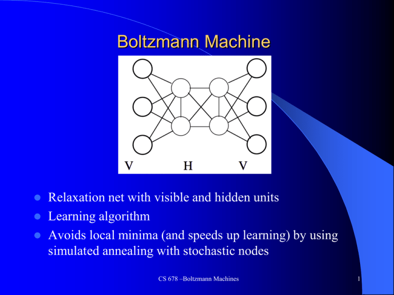
Boltzmann Machine



Relaxation net with visible and hidden units
Learning algorithm
Avoids local minima (and speeds up learning) by using
simulated annealing with stochastic nodes
CS 678 –Boltzmann Machines
1
Node activation: Logistic Function

Node k outputs sk = 1 with probability

else 0, where T is the temperature parameter
 Node does asynchronous random update
CS 678 –Boltzmann Machines
2
Network Energy and Simulated Annealing


Energy is like in the Hopfield Network
Simulated Annealing during relaxation
– Start with high temperature T (more randomness and large jumps)
– Progressively lower T while relaxing until equilibrium reached
– Escapes local minima and speeds up learning
Energy = -å wij si s j - åq i si
i¹ j
CS 678 –Boltzmann Machines
i
3
Boltzmann Learning





Physical systems at thermal equilibrium obey the
Boltzmann distribution Pa
-(Ea -E b )/T
=e
Pb
P+(Vα) = Probability that the visible nodes (V) are in state α
during training
P-(Vα) = Probability that the V is in state α when free
Goal: P-(Vα) ≈ P+(Vα)
What are the probabilities for all states assuming the
following training set (goal stable states)?
1001
1110
1001
0000
CS 678 –Boltzmann Machines
4
Boltzmann Learning

Information Gain (G) is a measure of the similarity
between P-(Vα) and P+(Vα)
+
P
(Va )
+
G = å P (Va )ln P (Va )


G = 0 if the probabilities are the same, else positive
Thus we can derive a gradient descent algorithm for weight
change by taking the partial derivative and setting it
negative
where pij = probability that nodei and nodej simultaneously
output 1 when in equilibrium
CS 678 –Boltzmann Machines
5
Network Relaxation/Annealing

A network time step is a period in which each node has updated
approximately once
1. Initialize node activations (Input)
– Hidden nodes activations initialized randomly
– Visible nodes
 Random
 Subset of nodes set to initial state, others random
 Subset of nodes clamped, others set to random or initial state
2.
3.
4.
Relax following an annealing schedule. For example:
2@30, 3@20, 3@10, 4@5
*Gather stats for m (e.g. 10) time steps, pij = #times_both_on/m
Set final node state (output) to 1 if it was a 1 during the majority of
the m time steps (could also output the probability or net value)
CS 678 –Boltzmann Machines
6
Boltzmann Learning Algorithm
Until Convergence (Δw < ε)
For each pattern in the training set
Clamp pattern on all visible units
Anneal several times calculating p+ij over m time steps
end
Average p+ij for all patterns
Unclamp all visible units
Anneal several times calculating p-ij over m time steps
Update weights: Δwij = C(p+ij - p-ij)
End
CS 678 –Boltzmann Machines
7
4-2-4 Simple Encoder Example

Map single input node to a single output
node
 Requires ≥ log(n) hidden nodes
1. Anneal and gather p+ij for each pattern
twice (10 time steps for gather). Noise .15
of 1 to 0, .05 of 0 to 1.
Annealing Schedule: 2@20,2@15,2@12,4@10
2. Anneal and gather p-ij in free state an equal
number of times
3. Δwij = 2 (p+ij – p-ij )
 Average: 110 cycles
CS 678 –Boltzmann Machines
8



4-2-4 Encoder
weights before and
after training
Note common
recursive weight
representation
What is the
network topology?
CS 678 –Boltzmann Machines
9


Shifting network, ~9000 cycles
Note no explicit I/O directionality
CS 678 –Boltzmann Machines
10
Boltzmann Learning

But does this Boltzmann algorithm learn the XOR function
 Hidden nodes
 But first order weight updates (ala perceptron learning rule)
CS 678 –Boltzmann Machines
11
Boltzmann Summary





Stochastic Relaxation – minima escape and learning speed
Hidden nodes and a learning algorithm, improvement over
Hopfield
Slow learning algorithm but need to extend to learn higher
order interactions
A different way of thinking about learning – creating a
probabilistic environment to match goals
Deep learning will use the Boltzmann machine
(particularly the restricted Boltzmann machine) as a key
component
CS 678 –Boltzmann Machines
12