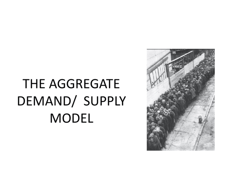
THE AGGREGATE
DEMAND/ SUPPLY
MODEL
The U.S. Great Depression
• 1929-1939
– Output fell by 30%
– Unemployment as high as 25%
– Prices declined 30% in the first four years
• Led to the development of modern
macroeconomic theory
Video
9-2
Before: Classical Economics
• Focused on long-run issues--growth
• Self-regulating markets through the “invisible hand”
– Prices would adjust during recessions
– Economy would always return to its potential output in the
long-run
• Depression caused by institutions that prevented prices
from falling, specifically:
– Labor unions
– Government
• Advocated a laissez-faire (hands-off) economic
policy
9-3
After: Keynesian Economics
• John Maynard Keynes in The General Theory of
Employment, Interest, and Money (1936)
• Problems of the Depression required a short-run,
rather than long-run, focus.
9-4
Keynesian Economics
• Adjustments to equilibrium for a single market and the
aggregate economy are different.
• Short-run equilibrium income may differ from long-run
potential income.
• Paradox of thrift
– In long run, saving leads to investment and growth.
– In short run, saving may lead to a decrease in
spending, output, and employment.
• Aggregate demand management by government may be
9-5
necessary.
Keynesian Economics and the AS/AD
Model
• Aggregate Demand Curve (AD)
– Relates changes in the price level to changes in aggregate expenditures =
C + I + G + (X-M)
• Short-Run Aggregate Supply Curve (SAS)
– Relates changes in the price level to changes in aggregate supply.
• Long-Run Aggregate Supply Curve (LAS)
– Shows potential output at any point in time
9-6
The Aggregate Demand Curve
Wealth, interest rate, and international
effects
P0
Multiplier effect
P1
AD
9-7
Y0 Y1
Ye
Real output
Shifts in the AD Curve
Initial effect = 100 increase in expenditures
Price
level
Multiplier
effect = 200
Change in total
expenditures = 300
P0
100
200
AD0
9-8
AD1
Real output
The Short-Run Aggregate Supply
Curve
Price level
SAS
Real output
9-9
Shifts in the SAS Curve
SAS1
1. Higher input prices
2. Higher import prices
Price level
3. Higher sales and excise
taxes
4. Reduced productivity
SAS0
Real output
9-10
Long-Run Aggregate Supply Curve
LAS
LAS1
• LAS curve shows potential output
• Vertical because potential output
Price Level
is unaffected by the price level.
• Increases in capital, resources,
Potential
output
Real output
9-11
growth-compatible institutions,
technology, and entrepreneurship increase potential output
and shift LAS to the right.
LAS Curve
LAS
• Potential output is assumed to be the
middle of a range bounded by high
and low levels of potential output.
C
• When resources are over-utilized
Price Level
B
A
Underutilized
resources
(point C), factor prices may be bid
up
SAS
When resources are under-utilized
(point A), factor prices may be bid
down
Overutilized
resources
• When LAS = SAS (point B), there is
Low-level
potential
output
9-12
High-level
potential
output
Real
output
no pressure for prices to rise or fall.
Short-Run Equilibrium:
Changes in AD
• Short-run equilibrium is
Price level
where SAS = AD0 (point
E).
SAS
P1
P
P00
F
E
AD1
AD0
Y
Y00
9-13
Y1
Real output
• If AD increases to AD1,
equilibrium output
increases to Y1 and the
price level increases to P1.
Short-Run Equilibrium:
Changes in SAS
Price level
• Short-run equilibrium is
SAS1
G
P1
SAS0
E
P0
AD
Y1
9-14
Y0
Real output
where SAS0 = AD (point
E). Equilibrium output is
Y0 and the price level is
P0.
• If SAS increases to SAS1,
equilibrium output
decreases to Y1 and the
price level increases to P1
(point G).
Long-Run Equilibrium
Price
level
LAS
• Long-run equilibrium is
H
P1
P0
point E where AD0 = LAS.
Equilibrium output is at
potential output YP and
the price level is Po.
E
AD1
AD0
YP
9-15
Real output
• An increase in AD to AD1
increases the price level
to P1 but output is unchanged at YP.
Integrating Short-Run and LongRun Frameworks
• The economy is in long-run
Price level
LAS
E
and short-run equilibrium at
point E where AD=SAS=LAS
and output is YP and the price
level is P0.
SAS
• AD grows at the same rate
P0
AD
9-16
YP
Real output
as potential output, so that
unemployment and inflation
are very low.
Recessionary Gap
• A recessionary gap is the
LAS
amount by which equilibrium
output is below potential output.
Price level
• At point A, some resources are
SAS0
A
P0
AD
Recessionary
gap
Y1
9-17
YP
Real output
unemployed and the recessionary
gap is YP – Y1.
Inflationary Gap
• An inflationary gap is the
Price level
LAS
amount by which equilibrium
output is above potential output.
• If the economy is at point C,
C
P0
SAS0
AD
Inflationary
gap
YP
9-18
Real
Y2 output
resources are being used
beyond their potential and the
inflationary gap is Y2 – YP.
Expansionary Fiscal Policy
Price
level
• Economy is at equilibrium
LAS
at A, there is a recessionary
gap Y0 – YP.
• Appropriate fiscal policy is
B
SAS
P1
P0
AD1
A
• AD increases to AD1 and
AD0
9-19
Y0
to increase government
spending and/or decrease
taxes.
YP
Real output
output returns to potential
output YP and prices
increase slightly to P1.
Contractionary Fiscal Policy
LAS
• Economy is at equilibrium at
Price level
B, there is an inflationary gap
Y2 – YP.
B
P2
• Appropriate fiscal policy is to
AS
AD0
AD2
YP
9-20
Y2 Real output
decrease government spending
and/or increase taxes.
• AD0 decreases to AD2 and
output returns to potential
output YP and inflation is
prevented.
Macro Policy Problems
• Implementing fiscal policy
– Slow legislative process
– Slow and uncertain reaction by the economy
• Avoiding “over-correcting”
9-21