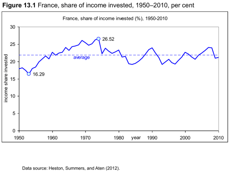
Figure 13.1 France, share of income invested, 1950–2010, per cent
France, share of income invested (%), 1950-2010
30
26.52
income share invested
25
average
20
16.29
15
10
5
0
1950
1960
1970
1980
Data source: Heston, Summers, and Aten (2012).
year
1990
2000
2010
Figure 13.2 Income levels and capital accumulation (Solow)
output
5
4
Equilibrium
capital available from
savings = investment
3
A
2
B
capital needed for
depreciation and
population growth
1
0
0
5
10
15
20
25
capital-labour ratio
k*
30
35
40
Figure 13.3 USA: GDP per capita, 1870-2010 (log scale)
USA; per capita GDP, 1870-2010 (log scale)
per capita GDP
100,000
10,000
1,000
1870
1890
1910
1930 year 1950
1970
1990
2010
Data sources: Maddison (2010) for the period 1870-2008, combined with Heston, Summers, and Aten (2012)
rgdpch for 2009 and 2010, normalized at 2008. Notes: measured in international 1990 Geary-Khamis $; the thin
line is a trend line
Figure 13.4 Income per capita and secondary schooling rate, 2010
GDP per capita and secondary schooling, 2010
GDP per capita (log scale)
100,000
Australia
10,000
1,000
Niger
100
0
20
40
60
80
100
secondary schooling rate (gross)
120
Data source: World Development Indicators online; GDP per capita measured in constant 2000 US $.
140
Figure 13.5 Income per capita and years of schooling; World Bank regions,
1960-2010
Years of schooling and per capita income
per capita income (log scale)
10,000
LAC
ECA
MENA
1,000
SSA
SA
EAP
100
0
1
2
3
4
5
6
7
8
9
years of schooling
Data sources: Cohen and Soto (2007) for years of schooling (population 15-64; population-weighted averages)
and World Bank Development Indicators online for per capita income (GDP in constant 2000 dollars); World Bank
regions (developing countries only) are: MENA = Middle East & North Africa; LAC = Latin America & Caribbean;
SSA = Sub-Sahara Africa; SA = South Asia; EAP = East Asia & Pacific; ECA = Eastern Europe & Central Asia;
data for 1960, 1970, 1980, 1990, 2000, 2010
Figure 13.6 Japan and Indonesia: income per capita, 1970-2010
Japan and Indonesia; per capita income 1870-2010
per capita income (log scale)
100,000
Japan
10,000
trendline Japan
trendline
Indonesia
1,000
100
1870
Indonesia
1890
Data sources: see Figure 13.3.
1910
1930
1950 year 1970
1990
2010
Figure 13.7 Overview of technology spillovers in an open developing economy
North 1
North 2
FDI14
FDI13
FDI24
Trade13
Trade24
Trade14 a
Trade23
South 3
E3
South 4
education
d -related
b
FDI23
Trade34
North-South
trade-related
spillover
E4
c
spillover
South-South traderelated spillover
b
North-South
FDI-related
spillover
Figure 13.8 Intertemporal adjustments in Singapore, 1972–2010, current
account balance, per cent of GDP
current account balance
Singapore; current account balance, 1972-2010 (% of GDP)
28.73
30
20
10
0
1970
1975
1980
1985
1990
-10
-20
1995
2000
2005
2010
year
-19.58
-30
Data source: World Bank development indicators online
Figure 13.9 Rapid growth in Europe – Asia trade, 1500-1800
Number of ships sailing to Asia from Europe, 1500-1800
3,000
2,500
2,000
1,500
1,000
500
0
1500-99
Portugal
1600-1700
Netherlands
England
1701-1800
France
Other
Data source: Maddison (2001); “Other” refers to ships of the Danish, Swedish trading companies, and the Ostend
company
Figure 13.10
Multinational trade
composition
a. Portugal; Estado da India (per cent by weight)
80
60
1513-19
40
1608-10
20
0
Pepper
Moluccan
Spices
Other
Spices
Textiles
Indigo
Other
b. Netherlands; Dutch East India Company (VOC,per cent by value)
80
60
1619-21
40
1778-801
20
0
Pepper
Other Spices
Textiles &
Raw Silk
Coffee & Tea
Other
c. England; English East India Company (EIC, per cent by value)
80
60
1668-70
40
1758-60
20
0
Data source: Maddison (2001).
Pepper
Textiles
Raw Silk
Tea
Other
Figure 13.11 A Dutch ship in Nagasaki, 1859
Text (right to left): A long time ago the Dutch already
were very skilled in navigation, and Dutch ships
sailed around the world. The Dutch were very well
versed in shipbuilding and of how to use ships
profitably for foreign markets. They chose good
materials and worked like when building up stone
walls; they used iron nails and filled up cracks with
tar and hemp.
In the fourth month they sailed from their country
(from Indonesia, the journey from Indonesia lasted
much longer) and in the sixth month they arrived
here.
When (the ship arrives) in Nagasaki and the
cannons, which are placed side by side, are fired,
clouds appear and make the ship invisible. When the
smoke has risen, the sails that had been visible in
large numbers suddenly appear to have been rolled
up.
Upon departure they also fire cannons, and before
the smoke has risen they have already hoisted the
sails, astonishing the spectators.
Their manoeuvring is truly miraculously fast and
mysterious.
Oranda fune no zu, 1859. Artist, Yoshitora; Publisher,
Yokohama, Shimaya, 36.5 × 25.5 cm. Inv.nr.: NEHA
SC 477 nr. 31, IISG.
Figure 13.12 The Japanese economy, 1500–2008, GDP & exports, percent of
world total
Japan: GDP and exports, percent of world total
9
Portuguese
expelled
end of
shogun era
6
GDP
3
export
Portuguese
landing
0
1500
Dutch
landing
1600
treaty of
Kanagawa
1700
1800
WW II
1900
2000
Data sources: Maddison (2001, 2010) and World Development Indicators online for 2008 share of world exports
(in current US dollars).
Figure 13.13 Developments in Chinese income and trade flows, 1960–2011
Economic developments in China, 1960-2011
100
50
Export of goods and services (% of GDP, right scale)
10
25
GDP/cap (% of world
average, log scale, left)
GLF
CR
Mao
ER
1
1960
SP&TS
GR
0
1970
1980
1990
2000
2010
Data source: World Development Indicators online; GDP per capita measured in constant 2000 US dollars; GLF =
Great Leap Forward; CR = Cultural Revolution; Mao = Mao’s death; ER = Economic Reform; SP&TS = Student
protests on Tiananmen Square; GR = start Great Recession.
Figure 13.14 The Dupuit triangle
price
pmax
Dupuit triangle
A
p
demand
O
q
qmax quantity
Figure 13.15 Dynamic costs of trade restrictions
Welfare costs of an increase in trade restrictions
100
Romer expected costs
welfare costs (per cent)
88
dynamic costs
50
45
static costs =
Romer unexpected costs
25
17
8
0
0
T'1 = 0.20
T1 = 0.10
Source: van Marrewijk and Berden (2007)
1-exp(-T)
1