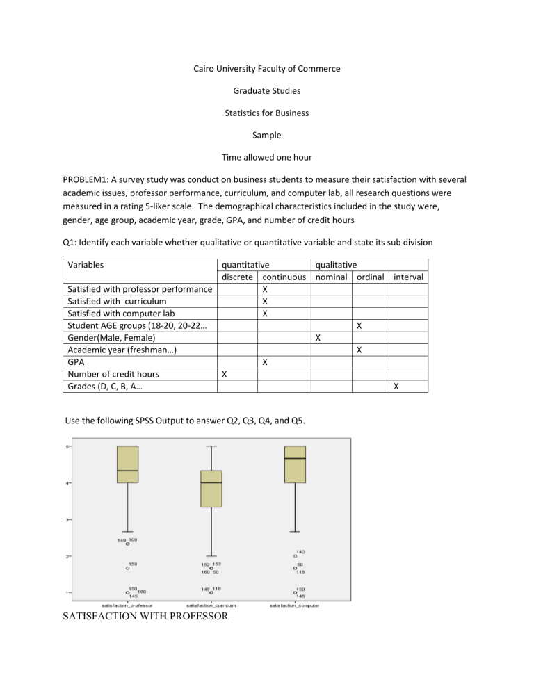
Cairo University Faculty of Commerce
Graduate Studies
Statistics for Business
Sample
Time allowed one hour
PROBLEM1: A survey study was conduct on business students to measure their satisfaction with several
academic issues, professor performance, curriculum, and computer lab, all research questions were
measured in a rating 5-liker scale. The demographical characteristics included in the study were,
gender, age group, academic year, grade, GPA, and number of credit hours
Q1: Identify each variable whether qualitative or quantitative variable and state its sub division
Variables
quantitative
qualitative
discrete continuous nominal ordinal interval
Satisfied with professor performance
X
Satisfied with curriculum
X
Satisfied with computer lab
X
Student AGE groups (18-20, 20-22…
X
Gender(Male, Female)
X
Academic year (freshman…)
X
GPA
X
Number of credit hours
X
Grades (D, C, B, A…
X
Use the following SPSS Output to answer Q2, Q3, Q4, and Q5.
SATISFACTION WITH PROFESSOR
The above boxplots illustrate the comparison between satisfactions of students with professor,
curriculum, and computer lab.
1: Which distribution has the largest number of outliers? Satisfaction with professor and the
curriculum
2: Describe each distribution, whether skewed to left, right, or symmetric.
A:SATISFIED WITH PROESSOR: SKEWED TORIGHT
B:SATISFIED WITH CURRICULM :SKEWED TO LEFT
C:SATISFIED WITH COMPUTER :Skewed to left
3: Which distribution has more variability?
Satisfaction with Curriculum
4: Which boxplot shows the highest median satisfaction?
Satisfaction with computer lab
5: Which distribution has the smallest lower inner fence?
4.
Problem2: The following tables provide 95% confidence intervals to the research questions.
One-Sample Statistics
N
Mean Std. Deviation
Std. Error Mean
satisfaction professor
160
4.24
.815
.064
Satisfaction curriculum
160
3.78
.888
.070
satisfaction computer
160
4.30
.843
.067
One-Sample Test
Test Value = 0
95% Confidence Interval of the Difference
t
satisfaction professor
df
Sig. (2-tailed) Mean Difference
Lower
Upper
65.758
159
.000
4.238
4.11
4.36
Satisfaction curriculum 53.778
159
.000
3.777
3.64
3.92
satisfaction computer
159
.000
4.296
4.16
4.43
64.489
Q1: Explain what the confidence interval of the research variables, say about their means
satisfaction?
Of Preprocessor, of Curriculum, of Computer lab
.
Research
Variables
95%
Confidence
Interval
Explanation
satisfaction
professor
Satisfaction
curriculum
satisfaction
computer
Q2: Test at 5% level whether students are satisfied with professor performance?
𝐻0 : The average satisfaction is less than or equal (3=neutral)
VS
𝐻𝑎 : The average satisfaction is more than (3 =neutral)
Is the hypothesis one tailed or two-tailed test?
What is the test statistic= t = _______
What the P-value_________
At𝛼 = 5% 𝑙𝑒𝑣𝑒𝑙 𝑜𝑓 𝑠𝑖𝑔𝑛𝑖𝑓𝑖𝑐𝑎𝑛𝑡, what is your decision regarding student satisfaction with
professor?
Q3: If I reject the above hypothesis that the average rating is 3 or less, when in fact it is 3 or less,
then, I committed
(a) Type I, error
(b) Type II, error
Q4: What is the power of the test means? Check one of the following
-Is the probability of rejecting that the average is more than 3, when in fact the average is more
than 3
-Is the probability of not rejecting that the average is 3, when infect it is 3.
-Is the probability of rejecting that the average satisfaction is less than or equal 3, when in fact it
is less than or equal three.
-Is the probability that we reject, the average is less than or equal 3,
Problem 3: The following output compares the research variables against their gender (male,
female). Answer Questions:
Independent Samples Test
Levene's Test
for Equality
of Variances
satisfaction
professor
Satisfaction
curriculum
satisfaction
computer
Equal
variances
assumed
Equal
variances
not
assumed
Equal
variances
assumed
Equal
variances
not
assumed
Equal
variances
assumed
Equal
variances
not
assumed
t-test for Equality of Means
Mean
Difference
Std. Error
Difference
95%
Confidence
Interval of the
Difference
Lower Upper
F
Sig.
t
1.332
0.25
2.234
158
0.027
0.285
0.128
0.033
0.538
2.268
158
0.025
0.285
0.126
0.037
0.534
1.445
158
0.15
-0.203
0.141
-0.481
0.074
1.455
156.431
0.148
-0.203
0.14
-0.479
0.073
0.928
158
0.355
-0.124
0.134
-0.388
0.14
-0.93
154.083
0.354
-0.124
0.134
-0.388
0.14
0.414
0.274
0.521
0.601
df
Sig.
(2tailed)
Q1: Test if any significant differences between males variance and females variance in their
satisfaction with Professor, curriculum, and computer lab.
Testing for equality of variances: From the output
Do male’s population and female population have the same variances: What is the p-value of the
test?
What are the p-values of the tests? Take the decisions at 5% level
P-values Decision at 5% level
1. Profess Satisfaction ____________
2. Curriculum Satisfaction__________
3. Computer Lab Satisfaction
Q2: Test for any significant difference between mean satisfactions of Males and Females and
their perceptions to the research questions. What are the p-values of these tests? Take the
decisions at 5% level
P-values Decision at 5% level
4. Professor Satisfaction ____________
5. Curriculum Satisfaction__________
6. Computer Lab Satisfaction
1. ) support the same decision of the t-test (Comparing two means) above?
Explain
Problem 4:
A possible Type II error would be to:
(a) Conclude that the students are less fit (on average) than the general population when in fact
they have equal fitness on average, .
(b) Conclude that the students have the same fitness (on average) as the general population when
in fact they are less fit on average.
(c) Conclude that the students have the same fitness (on average) as the general population when
in fact they are the same fitness level on average.
(d) Conclude that the students are less fit (on average) than the general population, when, in fact,
they are less fit on average.
(e) Conclude that the students have the same fitness (on average) when in fact they are more fit
on average.
Problem 5: We want to test H0 : µ = 1.5 vs. H1 : µ ≠ 1.5 at α= .05 . A 95% confidence interval
for µ calculated from a given random sample is (1.4, 3.6). Based on this finding we:
(a) Fail to reject H0 .
(b) Reject H0 .
(c) Cannot make any decision at all because the value of the test statistic is not available.
(d) Cannot make any decision at all because the distribution of the population is unknown.
(e) Cannot make any decision at all because (1.4, 3.6) is only a 95% confidence interval for µ .
Problem6:
In order to compare two kinds of feed, thirteen pigs are split into two groups, and each group
received one feed. The following are the gains in weight (kilograms) after a fixed period of time:
Feed A: 8.0 7.4 5.8 6.2 8.8 9.5
Feed B: 12.0 18.2 8.0 9.6 8.2 9.9 10.3
T
Group Statistics
Feeds
gains
N
Mean
Std. Deviation
Std. Error Mean
1
6
7.6167
1.44557
.59015
2
7
10.8857
3.49401
1.32061
Independent Samples Test
Levene's Test for
Equality of
Variances
F
Sig.
t-test for Equality of Means
t
df
Sig.
Mean
Std. Error
95% Confidence Interval
(2-
Differenc
Differenc
of the Difference
tailed)
e
e
Lower
Upper
gains Equal variances
1.600
.232
-2.130-
11
.057 -3.26905-
1.53464
-6.64676-
.10866
-2.260-
8.24
.053 -3.26905-
1.44648
-6.58770-
.04961
assumed
Equal variances
not assumed
1