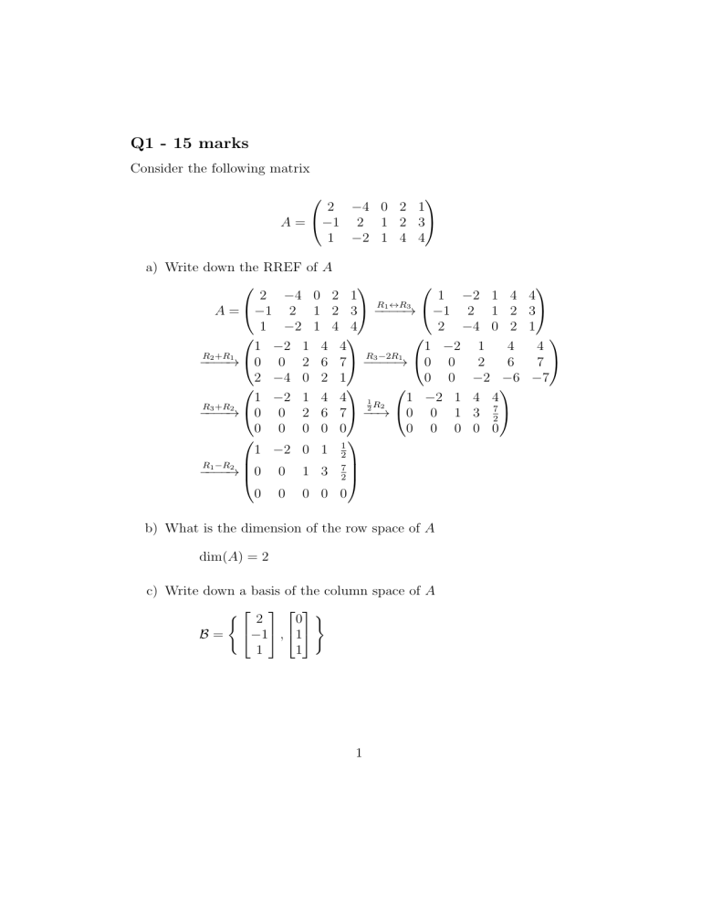
Q1 - 15 marks
Consider the following matrix


2 −4 0 2 1
A = −1 2 1 2 3
1 −2 1 4 4
a) Write down the RREF of A



2 −4 0 2 1
1 −2 1 4
R1 ↔R3



A = −1 2 1 2 3 −−−−→ −1 2 1 2
1 −2 1 4 4
2 −4 0 2



1 −2 1 4 4
1 −2 1
4
R +R1
R3 −2R1
0 0 2 6 7 −
2
6
−−2−−→
−−−→ 0 0
2 −4 0 2 1
0 0 −2 −6




1 −2 1 4 4
1 −2 1 4 4 1 R
2
R +R2
0 0 1 3 7 
0 0 2 6 7 −2−→
−−3−−→
2
0 0 0 0 0
0 0 0 0 0


1 −2 0 1 21

R −R2 
0 0 1 3 7 
−−1−−→
2

0 0 0 0 0
b) What is the dimension of the row space of A
dim(A) = 2
c) Write down a basis of the column space of A
(  2  0 )
B = −1 , 1
1
1
1

4
3
1

4
7
−7
d) What is the nullity of A. Write down a basis of the nullspace A?
nullity(A) = 3
From a):


1 −2 0 1 21 | 0


0 0 1 3 7 | 0
2


0 0 0 0 0 | 0
+ x4 + 12 x5 = 0
x1 − 2x2
x3 + 3x4 + 72 x5 = 0
x1 = 2s − t − 12 u
x2 =
s
x3 = −3t + 72 u
x4 =
t
x5 =
u
 
 
 1
2
−1
−2
1
0
 0 
 
 
 7 
 
 

⃗x = s 
0 + t −3 + u  2 
0
1
 0 
0
0
1
     1 
2
−1
− 


     2 


1  0   0 

7 





∴ B = 0 , −3 ,  2 



0  1   0 






0
1
0
2
Q2 - 20 marks
The aim of this question will be to produce matrices with specificed eigen
values which are not just triangular! Let p(x) be the polynomial
p(x) = xn + an−1 xn−1 + · · · + a1 x + a0
and define the companion matrix to the polynomial as


−an−1 −an−2 · · · −a1 −a0
 1
0
···
0
0 



..
.. 
..
C(p) =  0
.
1
.
. 


 0
0
···
0
0 
0
0
···
1
0
a) Write down the matrix C(p) of the polynomial p(x) = x3 − 4x2 + 5x − 2


4 −5 2
C(p) = 1 0 0
0 1 0
b) Find the characteristic polynomial of the matrix C(p) which you wrote
in the previous step


4 − λ −5 2
−λ 0 
C(p) − λI =  1
0
1 −λ
det(C(p) − λI = 2
1 −λ
4 − λ −5
−λ
0 1
1
−λ
= 2(1) − λ[(4 − λ)(−λ) − (−5)]
= 2 − λ(−4λ + λ2 + 5)
= 2 + 4λ2 − λ3 − 5λ
= −λ3 + 4λ2 − 5λ + 2 = 0
3
 
4

c) Show that 2 is an eigenvector of C(p) with eigenvalue 2
1
 
4
Let ⃗x be 2, then
1

  
  
4 −5 2
4
16 − 10 + 2
8







2 =
4
C(p)⃗x = 1 0 0
= 4
0 1 0
1
2
2
   
4
8



λ⃗x = 2 2 = 4
1
2
∴ C(p)⃗x = λ⃗x
 
4

∴ ⃗x = 2 is an eigenvector of C(p) with eigenvalue λ = 2
1
d) Find the matrix C(p) associated to the polynomial p(x) = x3 + ax2 +
bx + c


−a −b −c
0
0
C(p) =  1
0
1
0
4
e) Determine the characteristic polynomial of the matrix C(p) from the
previous step


−a − λ −b −c
−λ 0 
C(p) − λI =  1
0
1 −λ
det(C(p) − λI) = −1
−a − λ −c
−a − λ −b
−λ
1
0
1
−λ
= −1[(−a − λ)(0) − (−c)(1)] − λ[(−a − λ)(−λ) − (−b)(1)]
= −1(c) − λ(aλ + λ2 + b)
= −c − aλ2 − λ3 − bλ
= −λ3 − aλ2 − bλ − c = 0
5
f) Show
 2 that if λ is an eigenvalue of the companion matrix C(p), then
λ
 λ  is an eigenvector of C(p) corresponding to λ
1
Eλ = Nul(C(p) − λI)




−a − λ −b −c | 0
−a − λ −b −c | 0
R ↔R3
 0
−λ 0 | 0 −−2−−→
1 −λ | 0
= 1
0
1 −λ | 0
1
−λ 0 | 0


1
−λ 0 | 0
R1 ↔R3

0
1 −λ | 0
−−−−→
−a − λ −b −c | 0


1
0
−λ2
| 0
R3 +bR2
R +λR2
 0
1
−λ
| 0
−−1−−−→
−a − λ 0 −c − bλ | 0


1 0
−λ2
| 0
R3 +(a+λ)R1
−λ
| 0
−−−−−−−→ 0 1
3
2
0 0 −λ − aλ − bλ − c | 0
From the characteristic polynomial: λ3 = −aλ2 − bλ − c


1 0
−λ2
| 0
−λ
| 0
∴ 0 1
2
2
0 0 −(−aλ − bλ − c) − aλ − bλ − c | 0


1 0 −λ2 | 0
x1
− λ2 x3 = 0
∴ 0 1 −λ | 0 ⇒
x2 − λx3 = 0
0 0 0 | 0
x1 = λ 2 s
x2 = λs
⇒
 2
λ

⃗x = s λ 
1
x3 = s
 2 
 λ 
∴ BEλ =  λ 


1
 2
λ
⇒  λ  is an eigenvector of C(p) corresponding to λ
1
6
g) Construct a non-triangular 3 × 3 matrix of eigenvalues -2, 1, 3 using
companion matrices. Briefly justify your answer.
From f)
 2
λ

Eλ = λ 
1
Thus,
λ = −2, 1, 3
 
 
4
1
BE−2 = −2
BE1 = 1
1
1


4 1 9
∴ P = −2 1 3
1 1 1


4 1 9 | 1 0 0
[ P | I ] = −2 1 3 | 0 1 0
1 1 1 | 0 0 1


3 0 8 | 1 0 −1
R1 −R3
R −R3
−3 0 2 | 0 1 −1
−−2−−→
1 1 1 | 0 0 1


3 0 8 | 1 0 −1
R +R1
0 0 10 | 1 1 −2
−−2−−→
1 1 1 | 0 0 1


3
0
8
|
1
0
−1
1
R2
1
1
−2 
−10
−−→ 0 0 1 | 10
10
10
1 1 1 | 0 0 1


2
−8
6
3 0 0 | 10
10
10

R1 −8R2 
1
1
−2 

−−−−→ 0 0 1 | 10 10 10 
1 1 1 | 0 0 1
7
BE3
 
9
= 3
1

2
1 0 0 | 30

−−−−→ 
1 1 1 | 0
3
0 0 1 | 30

2
1 0 0 | 30
R −R1 
0 1 1 | −2
−−2−−→
30

3
0 0 1 | 30

2
1 0 0 | 30
R −R3 
0 1 0 | −5
−−2−−→
30

3
0 0 1 | 30

1
−4
1 0 0 | 15
15

1
−1
→
− 
6
0 1 0 | 6
1
1
0 0 1 | 10
10

 1
4
1
−
15
15
5


−1  1
1
1 
P − 6
6

1
1
1
−5
10
10
R2 ↔R3
1
R
3 1
A = P DP −1


4 1 9
−2
= −2 1 3  0
1 1 1
0
 1


−8 1 27  15
1

4 1 9 
=
− 6
−2 1 3
1
10


2 5 −6
A = 1 0 0 
0 1 0
−8
30
6
30


1

0
3
30
−6
30
−8
30
8
30
3
30
6
30

24 
30 
−6
30
−8
30
5
30
3
30
6
30
1
5



1

−6
30


1

−1
5

 1
4
1

−
15
15
5
0 0 

1
1

1 0 
−
1
6
6


0 3
1
1
1
−
10
5
 10
4
1
− 15 5

1

1
6

1
1
−5
10
8
Q3 - 20 marks
Consider the matrix


0 0
4
2 0
0

0 −2 0 
0 0 −2
2
0
A=
0
0
a) Find matrices P and D (with D diagonal) so that A = P DP −1
CA (λ) = (λ − 2)2 (λ + 2)2
λ = 2, −2
For λ = 2,


0
0
4
2−2
0
0 

0
−2 − 2
0 
0
0
−2 − 2

0
4
0
0

−4 0 
0 −4

0 0 0
4 |
0 0 0
0 |
E2 = Nul(A − 2I) = 
0 0 −4 0 |
0 0 0 −4 |
2−2
 0
A − 2I = 
 0
0

0 0
0 0
=
0 0
0 0
1
R
4 1
R1 ↔R2
− 41 R3
− 14 R4

0
0
−−−−→ 
0
0
0
0
0
0
0
0
1
0
0
1
0
1
|
|
|
|


0
0
R3 ↔R1

0
−R1 0
 −R−4−
−→ 

0
0
0
0
x1 = free
x1 = s
x2 = free
x2 = t
x3 = 0
x3 = 0
x4 = 0
x4 = 0
9

0
0

0
0
⇒

1 0 | 0
0 1 | 0

0 0 | 0
0 0 | 0
 
 
1
0
0
1

 
⃗x = s 
0 + t 0
0
0
0
0
0
0
∴ BE2
   
0 

 1


0 1




=  , 
0
0 





0
0
For λ = −2,

4
0
A + 2I = 
0
0
0
4
0
0
0
0
0
0

4
0

0
0

E−2
4
0
= N ul(A + 2I) = 
0
0
x1 + x4 = 0
0
4
0
0
0
0
0
0
1
0
Thus, P = 
0
0
0
1
0
0
|
|
|
|
x1 = −t
x2 = 0
x2 = 0
x3 = free
x3 = s
x4 = free
x4 = t
   
0
−1 


   

0
, 0 
∴ BE−2 = 
1  0 





0
1

4
0
0
0


0 −1
2


0 0
0
and D = 
0
1 0
0 1
0
10
⇒


1 0 0 1
0 41 R1
1


R
0 4 2 0 1 0 0
−−→ 
0 0 0 0
0
0 0 0 0
0
 
 
0
−1
0
0

 
⃗x = s 
1 + t  0 
0
1

0 0
0
2 0
0

0 −2 0 
0 0 −2
|
|
|
|

0
0

0
0
b) For each positive integer n, write down a formula for An
∀n ∈ Z+ ,
An = (P DP −1 )n
−1
−1
= (P D
P
)( P D
P
) . . . ( P DP −1 ) = P Dn P −1

 n

1 0 0 −1
2
0
0
0
1
0 1 0 0   0 2 n


0
0  0

=
0 0 1 0   0 0 (−2)n
0  0
0 0 0 1
0 0
0
(−2)n
0
11
0
1
0
0
0
0
1
0

1
0

0
1
Q4 - 20 marks
A study of pine nuts in the American southwest from 1940 to 1947 hypothesized that nut production followed a Markov chain. The data suggested
that if one year’s crop was good, then the probabilities that the following
year’s crop would be good, fair, or poor were 0.08, 0.07, 0.85 respectively; if
one year’s crop was fair, then the probabilities that the following year’s crop
would be good, fair, or poor were 0.09, 0.11, and 0.80, respectively; if one
year’s crop was poor, then the probabilities that the following year’s crop
would be good, fair, or poor were 0.11, 0.05, 0.84 respectively.
a) Write down the transition matrix for this Markov process


0.08 0.09 0.11
A = 0.07 0.11 0.05
0.85 0.80 0.84
b) If the pine cut crop was good in 1940, find the probabilities of a good
crop in the years 1941 through 1945
  
  

1
0.08 0.09 0.11
1
0.08
1941: A 0 = 0.07 0.11 0.05 0 = 0.07 ⇒ 0.08
0
0.85 0.80 0.84
0
0.85
 
 


1
1
0.08
2 



1942: A 0 = AA 0 = A 0.07
0
0
0.85


 

0.08 0.09 0.11
0.08
0.1062
= 0.07 0.11 0.05 0.07 = 0.0558
0.85 0.80 0.84
0.85
0.838
⇒ 0.1062


 
 
1
0.1062
1
1943: A3 0 = AA2 0 = A 0.0558
0.838
0
0


 

0.08 0.09 0.11
0.1062
0.105698
= 0.07 0.11 0.05 0.0558 = 0.055472
0.85 0.80 0.84
0.838
0.83883
⇒ 0.105698
12
 
 


1
1
0.105698
1944: A4 0 = AA3 0 = A 0.055472
0
0
0.83883


 

0.08 0.09 0.11
0.105698
0.10571962
= 0.07 0.11 0.05 0.055472 = 0.05544228
0.85 0.80 0.84
0.83883
0.8388381
⇒ 0.10571962
 
 


1
1
0.10571962
1945: A5 0 = AA4 0 = A 0.05544228
0
0
0.8388381



0.08 0.09 0.11
0.10571962
= 0.07 0.11 0.05 0.05544228
0.85 0.80 0.84
0.8388381


0.1057195658

= 0.0554409292 ⇒ 0.10571962
0.838839505
c) In the long run, what proportion of the crops will be good, fair, and
poor?
Since the steady state vector is the eigenvector corresponding to λ = 1,


0.08 − 1
0.09
0.11
| 0
0.11 − 1
0.05
| 0
E1 = Nul(A − 1I) =  0.07
0.85
0.80
0.84 − 1 | 0


−0.92 0.09
0.11 | 0
=  0.07 −0.89 0.05 | 0
0.85
0.80 −0.16 | 0


9
11
−
|
0
1
−
1
92
92
R
−0.92 1
−−−−→ 0.07 −0.89 0.05 | 0
0.85 0.80 −0.16 | 0


9
1 − 92
− 11
|
0
92
R2 −0.07R1

R3 −0.85R1 
325
537

−−−−−−→ 0 − 368 9200 | 0

325
537
0 368 − 9200 | 0
13

11
− 92
| 0

R +R1 
0 − 325 537 | 0
−−3−−→
368
9200


0
0
0 | 0


9
1 − 92
− 11
|
0
92

− 368
R 
325 2 
537
−−−−→ 0 1 − 8125 | 0

0 0
0
| 0


1024
1 0 − 8125
| 0
9

R2 
R1 + 92
537

0
1
−
|
0
−−−−
−→ 
8125


0 0
0
| 0

x1
1
−
x2 −
a
9
− 92
1024
x
8125 3
537
x
8125 3
x2 =
1024
s
8125
537
s
8125
x3 =
s
x1 =
=0
=0
 1024 
8125
⇒
 537 

⃗x = s 
 8125 
1
537
8125
1024
+a
+a=1⇒a=
8125
8125
9686
 1024   512 
8125
4838
 537   537 

 
⇒ ⃗v = a 
 8125  =  9686 
8125
1
9686
512
∴ In the long run, 4838
crops will be good,
8125
crops
will
be
poor
9686
14
537
9686
crops will be fair, and