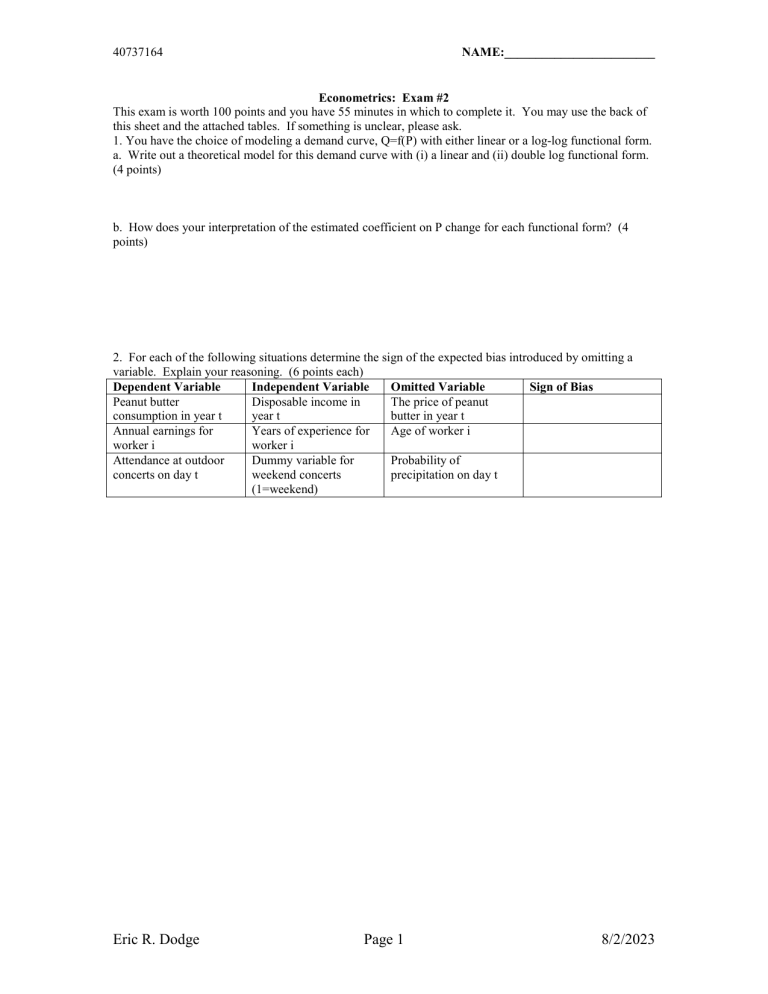
40737164
NAME:________________________
Econometrics: Exam #2
This exam is worth 100 points and you have 55 minutes in which to complete it. You may use the back of
this sheet and the attached tables. If something is unclear, please ask.
1. You have the choice of modeling a demand curve, Q=f(P) with either linear or a log-log functional form.
a. Write out a theoretical model for this demand curve with (i) a linear and (ii) double log functional form.
(4 points)
b. How does your interpretation of the estimated coefficient on P change for each functional form? (4
points)
2. For each of the following situations determine the sign of the expected bias introduced by omitting a
variable. Explain your reasoning. (6 points each)
Dependent Variable
Independent Variable
Omitted Variable
Sign of Bias
Peanut butter
Disposable income in
The price of peanut
consumption in year t
year t
butter in year t
Annual earnings for
Years of experience for
Age of worker i
worker i
worker i
Attendance at outdoor
Dummy variable for
Probability of
concerts on day t
weekend concerts
precipitation on day t
(1=weekend)
Eric R. Dodge
Page 1
8/2/2023
40737164
3.
a.
b.
c.
NAME:________________________
Explain the following concepts and how you can identify them. (6 points each)
A dominant independent variable.
An irrelevant independent variable.
A redundant independent variable.
4. A cross-sectional regression was run on a sample of 44 states in an effort to understand federal defense
spending by state (standard errors in parentheses):
Sˆi  148.0  .841Ci  .0115Pi  .0078Ei
(.027)
(.1664)
(.0092)
where: Si = annual spending (millions of dollars) on defense in the ith sate
Ci = contracts (millions of dollars) awarded in the ith state (contracts are often for many years of
service) per year
Pi = annual payroll (millions of dollars) for workers in defense-oriented industries in the ith state
Ei = the number of civilians employed in defense-oriented industries in the ith state.
a. Do all of the above coefficients match your expectations? Explain your reasoning. (4 points)
b. Calculate t-scores and test for significance of the above results at the 5% level. (6 points)
c. The VIFs for this equation are all above 20, and those for P and C are above 30. What conclusion does
this information allow you to draw? Explain. (6 points)
d. What recommendation would you make for a rerun of this equation with a different specification?
Explain your answer. (6 points)
Eric R. Dodge
Page 2
8/2/2023
40737164
NAME:________________________
5. The table below presents results from a model of the U.S. poverty rate as a function of the U.S.
unemployment rate (annual 1980-2003). Use this data to respond to the questions below.
Dependent Variable: POVERTY
Method: Least Squares
Date: 03/23/06 Time: 09:23
Sample: 1980 2003
Included observations: 24
Variable
Coefficient
Std. Error
t-Statistic
Prob.
C
UNEMPLOY
9.792052
0.586614
0.611186
0.094726
16.02138
6.192734
0.0000
0.0000
R-squared
Adjusted R-squared
S.E. of regression
Sum squared resid
Log likelihood
Durbin-Watson stat
0.635460
0.618890
0.676259
10.06116
-23.62207
0.323725
Mean dependent var
S.D. dependent var
Akaike info criterion
Schwarz criterion
F-statistic
Prob(F-statistic)
13.47917
1.095437
2.135173
2.233344
38.34995
0.000003
a. Is the coefficient on UNEMPLOY the sign you expected? Are you confident in the statistical
significance of this coefficient? Explain. (4 points)
b. Where are the indicators of econometric problems? Justify your answer with intuition, relevant statistics,
and hypothesis tests. (6 points)
c. Given your response in part (b) explain how you would re-estimate the model and how this would fix
the problems. (6 points)
Eric R. Dodge
Page 3
8/2/2023
40737164
NAME:________________________
6. The table below presents results from a cross-sectional model of housing prices (P) in Monrovia, CA as
a function of several characteristics of the house and neighborhood. Use this data to respond to the
questions below.
Dependent Variable: P
Method: Least Squares
Date: 03/23/06 Time: 13:50
Sample: 1 43
Included observations: 43
Variable
Coefficient
Std. Error
t-Statistic
Prob.
C
S
A
A^2
N
Y
182.3031
0.086373
-1.869710
0.015699
-29.89189
0.005334
33.62101
0.011137
0.906212
0.009524
4.928443
0.001469
5.422298
7.755401
-2.063215
1.648268
-6.065179
3.630397
0.0000
0.0000
0.0462
0.1078
0.0000
0.0009
R-squared
Adjusted R-squared
S.E. of regression
Sum squared resid
Log likelihood
Durbin-Watson stat
0.917860
0.906760
24.19658
21662.56
-194.7904
1.759940
Mean dependent var
S.D. dependent var
Akaike info criterion
Schwarz criterion
F-statistic
Prob(F-statistic)
242.3023
79.24150
9.339088
9.584836
82.69001
0.000000
Variables:
P = price (in $1000’s) of the ith house
S = size (in square feet) of the ith house
A = age of the ith house in years
A^2 = squared age of ith house
N = the quality of the neighborhood of the ith house (1 = best, 4 = worst) as rated by two local real estate
agents
Y = the size of the yard around the ith house (in square feet)
a. Given these results, do you suspect any problems with heteroskedastic errors in this model? Why or
why not? (6 points)
b. A White test has been conducted and the test statistic nR2 = 18.2. Using all squared and cross-terms
there were k=19 slope coefficients. Given this information, what can you say about the possibility of
heteroskedasticity in the model? (6 points)
c. Given your response in part (b) what kind of changes would you make to this model? Justify your
decision. (6 points)
Eric R. Dodge
Page 4
8/2/2023