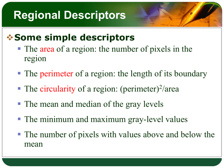
Regional Descriptors
Some simple descriptors
 The area of a region: the number of pixels in the
region
 The perimeter of a region: the length of its boundary
 The circularity of a region: (perimeter)2/area
 The mean and median of the gray levels
 The minimum and maximum gray-level values
 The number of pixels with values above and below the
mean
Moment-Based Shape Features
 Moments are statistical measures of data to describe
objects after segmentation.
Simple properties which are found via moments include
area, its centroid, and orientation.
– Order 0 is just the number of points in the data.
– Order 1 is the sum and is used to find the average.
– Order 2 is related to the variance, and order 3 to the skew.
Higher orders can also be used, but don’t have simple
meanings.
Central Moments
The central moments are defined as :
 pq  



 
( x  x ) p ( y  y ) q f ( x, y)dxdy
For discrete binary images,
 pq   ( x  x ) p ( y  y ) q
x
y
Central Moments
 The zero-order moment,  00, is
00   ( x  x ) 0 ( y  y ) 0  Area
x
y
 Which represents the total mass of a function.
 The center of mass ( x , y ) can be calculated
1
x   x
n x y
1
y   y
n x y
 Where n is the number of object pixels
Moment Tensor
The orientation of the object is defined as
The eccentricity is the ratio of the distance between the
foci of the ellipse and its major axis length.
Geometrical Shape parameters
The perimeter is another geometrical parameter that can
easily be obtained from the chain code of the object
boundary.
Count the length of the chain code and take into
consideration the steps in diagonal directions are longer
by a factor of √2.
where ne and no are the number of even and odd chain
code steps, respectively.
Geometrical Shape parameters
Area and perimeter are two parameters that describe the
size of an object.
In order to compare objects observed from different
distances, it is important to use shape parameters that do
not depend on the size of the object.
The circularity c is one of the simplest parameters of this
kind.
Bounding Box is defined as the rectangle that is
large enough to contain all object pixels.
Problem
Is it possible to discriminate between varieties of grains using image analysis?
Texture Analysis
 How to discriminate the samples?
 Single grain analysis
– Measure size, roundness, colour etc. for each grain.
– Extraction of singe grain is difficult.
 Texture analysis
– Finds features for the texture of the image surface.
– Easy to implement.
– Several different features available.
Texture Analysis
What is texture?
Texture is an feature that can help to segment images
into regions of interest and to classify those regions.
Texture gives us information about the spatial
arrangement of the colors or intensities in an image.
Mathematical procedures to characterize texture fall
into two major categories,
1. Statistical
2. Syntactic
Statistical Methods
First-order (one pixel)
- properties of individual pixel values (average & variance)
- ignore the spatial interaction between image pixels
Second-order (two pixels)
- properties of two pixel values occurring at specific locations
relative to each other
- Co-occurrence matrices
Higher-order (three or more pixels)
- properties of more pixel values
Gray Level Co-occurrence Matrix
Gray Level Co-occurrence Matrix (GLCM) also called
Gray Tone Spatial Dependency Matrix introduced by
Haralick 1979.
GLCM is one of the most popular statistical approaches
in analysis of gray level tones in an image.
It considers a second order texture calculation that
measures the relationship between two neighboring
pixels at a time.
GLCM is created from a gray scale image.
GLCM
GLCM defines the probability that gray level i called the
reference pixel occurs at a distance d in direction θ from
gray level j called the neighboring pixel in the image.
The neighbor pixel is chosen to be
 Horizontal (0º)
 Vertical (90º)
 Diagonal
• Bottom left to top right (45º)
• Top left to bottom right (135º)
GLCM
So for each image, we can compute four symmetrical
GLCM matrices representing the four directions denoted
P0, P45, P90, and P135.
The GLCM is defined by:
P [i, j ]  nij
• where nij is the number of occurrences of the pixel i and its
neighbor j lying at distance d in the image.
• The co-occurrence matrix P has a dimension n× n,
• where n is the number of gray levels in the image.
GLCM Steps
Steps for creating a symmetrical normalized GLCM:
1. Create an empty framework matrix (n x n).
2. Decide the angle.
3. Count the occurrences and fill in the framework matrix.
4. Add the matrix to its transpose to make it symmetrical.
As example (0, 180)
5. Normalize the matrix to turn it into probabilities.
6. Repeat these steps for each angle.
GLCM Steps
1.
Compute number of gray pixel (n) in the image
to define framework matrix (n x n).
0
0
1
1
1
0
0
1
1
1
0
0
2
1
1
2
2
2
3
3
2
2
3
3
3
Image
framework matrix
(4 x 4)
GLCM Steps
2.
3.
Decide the angle
Computed first GLCM matrix => P0.
0
0
1
1
1
0
0
1
1
1
0
0
2
1
1
2
2
2
3
3
2
2
3
3
3
Image
3
2
1
0
0
5
0
0
0
1
3
2
0
0
0
3
framework matrix
(4 x 4)
GLCM Steps
4. Add the matrix to its transpose to make it symmetrical.
3
2
1
0
0
5
0
0
0
1
3
0
0
0
3
0
0
0
2
5
1
0
2
1
0
3
0
3
0
0
2
3
transpose
GLCM matrix
0 direction
GLCM matrix
180 direction
add
6
2
1
0
2
10
1
0
1
1
6
2
0
0
2
6
Symmetric GLCM
GLCM Steps
5. Finally for computing the probability of occurrence, we
normalize the symmetrical matrix by dividing each
element by the sum of all elements.
Normalized
GLCM
=
6
2
1
0
0.15
0.05
0.025
0
2
10
1
0
0.05
0.25
0.025
0
1
1
6
2
0.025
0.025
0.15
0.05
0
0
2
6
0
0
0.05
0.15
6. By the same way we can compute the other three
directions.
GLCM Example
GLCM Features
Haralick suggested a set of 14 textural features which
can be extracted from the co-occurrence matrix, and
which contain information about image textural
characteristics.
The most popular features :
1.
Contrast.
2.
Homogeneity.
3.
Entropy.