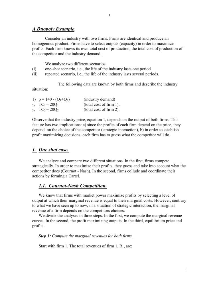
1
A Duopoly Example.
Consider an industry with two firms. Firms are identical and produce an
homogenous product. Firms have to select outputs (capacity) in order to maximize
profits. Each firm knows its own total cost of production, the total cost of production of
the competitor and the industry demand.
(i)
(ii)
We analyze two different scenarios:
one-shot scenario, i.e., the life of the industry lasts one period
repeated scenario, i.e., the life of the industry lasts several periods.
The following data are known by both firms and describe the industry
situation:
1) p = 140 - (Q1+Q2)
2) TC1 = 20Q1
3) TC2 = 20Q2
(industry demand)
(total cost of firm 1),
(total cost of firm 2).
Observe that the industry price, equation 1, depends on the output of both firms. This
feature has two implications: a) since the profits of each firm depend on the price, they
depend on the choice of the competitor (strategic interaction), b) in order to establish
profit maximizing decisions, each firm has to guess what the competitor will do.
1. One shot case.
We analyze and compare two different situations. In the first, firms compete
strategically. In order to maximize their profits, they guess and take into account what the
competitor does (Cournot - Nash). In the second, firms collude and coordinate their
actions by forming a Cartel.
1.1. Cournot-Nash Competition.
We know that firms with market power maximize profits by selecting a level of
output at which their marginal revenue is equal to their marginal costs. However, contrary
to what we have seen up to now, in a situation of strategic interaction, the marginal
revenue of a firm depends on the competitors choices.
We divide the analyses in three steps. In the first, we compute the marginal revenue
curves. In the second, the profit maximizing outputs. In the third, equilibrium price and
profits.
Step 1: Compute the marginal revenues for both firms.
Start with firm 1. The total revenues of firm 1, R1, are:
1
2
R1= pQ1 = (140-(Q1+Q2))Q1 = 140 Q1 - Q12 - Q2Q1.
The marginal revenue of firm 1, MR1, is just the derivative of the total revenues with
respect to Q1. Hence
5)
MR1 = 140- 2Q1 - Q2 (Marginal revenue of firm 1).
Similarly, the total revenues of firm 2, R2 are:
R2= pQ2 = (140-(Q1+Q2))Q2 = 140 Q1-Q2 2-Q2Q1.
Hence, the marginal revenue for firm 2, MR2, is:
6)
MR2 = 140- 2Q2 - Q1,
(Marginal revenue of firm 2)
Step 2: Compute the profit maximizing outputs for both firms.
To start with observe that equations 2) and 3) imply that MC1 =MC2 = 20.
Start with firm 1. Profit maximization for both firms entails selecting an output at which
the marginal revenue equates the marginal cost. Hence for firm 1, MR1 = MC1 implies by
equation 4):
140- 2Q1 - Q2 = 20
(Marginal revenue of firm 1)
or equivalently
6) Q1 = (120 - Q2 )/2
(Reaction function of firm 1, RF1)
Equation 6) is called a reaction function: it sets the profit maximizing value of firm 1’ s
output, Q1, for any value of the competitor output, Q2 .
Using the same argument, for firm 2, MR2 =MC2 implies by equation 4)
140- 2Q2 - Q1 = 20
(Marginal revenue of firm 2)
or equivalently
7) Q2 = (120 - Q1 )/2
(Reaction function of firm 2)
Hence, for given choices of the competitors, both firms use their reaction
functions to set profit maximizing quantities of their outputs. However, the game is
simultaneous and firms do not observe the actions selected by the competitor. Therefore,
how are they going to guess the competitor output? Each firm knows that everybody in
the market will try to maximize profits or, equivalently, that every firm will use its own
reaction function. Both firms can compute the solution (Q1*, Q2* ) to equations 6 and 7.
2
3
Given Q2*, firm 1 will maximize its profit by choosing Q1* and, given Q1*, firm 2 will
maximize its profit by choosing Q2*. In other words, the pair (Q1*, Q2*) constitutes a
Nash equilibrium: no firm has an incentive to take unilateral deviations.
In order to compute the pair (Q1*, Q1*), we need to solve equations 6 and 7.
However, a simple observation will simplify the computations. The two firms are
identical and, therefore, it must be that Q1*= Q2*. (more precisely, 6 and 7 are linear
equations symmetric in the indexes 1 and 2 ). Substituting the equation Q1* = Q2* into
equation 6 (or 7) we get:
Q1* = (120 - Q1* )/2
which together with Q1 *= Q2 * implies
Q1 *= Q2 * = 40
Hence, substituting Q1 *= Q2 * = 40 in the demand expression (equation 1)), we get
`
p*=140 -( Q1 *+ Q2 * ) = 60
Profits are:
A1* = p* Q1 * - 20 Q1 * = 60*40 - 20*40 = 1,600
A2* = p* Q2 * - 20 Q2 * = 60*40 - 20*40 = 1,600
1.2 Cartel
Suppose that both firms agree to form a cartel. The goal of the cartel is to set the
industry output at a level that maximizes industry profits. A rule governing the cartel
behavior specifies how the industry output and profits must be shared among the cartel
members. In our example, things are very simple. So we can safely assume that firms
equally share both profits and production. Let Q denote the industry output. Profits
maximization of the industry implies that the industry marginal revenue must equate the
industry marginal cost. Since by 1) demand is p = 140 -Q, the industry revenues are
R= pQ = (140-Q)Q = 140 Q - Q 2.
The industry marginal revenue, MR, is just the derivative of the industry total
revenues with respect to Q. Hence:
MR = 140- 2Q
Since both firms have the same constant marginal (and average) cost, the marginal cost of
the industry, MC, is equal to 20 (by equation 2) and 3)). Therefore, MR = MC implies
3
4
140- 2Q = 20
which implies that the profit maximizing industry output, QC , is
QC = 60
Substituting QC = 60 into the demand (equation 1) we get that
pC = 140 - QC = 140 - 60 = 80.
Each firm will therefore produce (and sell) half of the industry output (i.e, Q1 C = Q2 C
=30) realizing profits equal to:
A1C = pC Q1 C - 20 Q1 C = 80*30 - 20*30 = 1,800 ,
A2C = pC Q2 C - 20 Q2 C = 80*30 - 20*30 = 1,800.
Stability of the cartel
When acting according to the Cournot - Nash prediction, firms realize profits
equal to $1,600. When they form a cartel, they both realize profits equal to $1,800. Since
the goal of both firms is profit maximization, should we conclude that the existence of the
Cartel is the only sensible prediction of the one shot situation? The answer to this
question is negative. The cartel is intrinsically unstable: both firms have a unilateral
incentive to produce above the cartel agreement (i.e., above 30). In different words, the
cartel agreement does not constitute a Nash equilibrium and it is, therefore, vulnerable to
unilateral deviations.
To analyze this point more clearly, suppose that firm 2 credibly commits itself to
produce, according to the Cartel prescription, an output Q2C = 30. What is, given the
output choice of firm 2, the profit maximizing output of firm 1? From the previous
analysis, we know that firm 1 computes the profit maximizing output utilizing its own
reaction function. Therefore, the profit maximizing output, Q1, is obtained by substituting
Q2C = 30 into firm 1 reaction function, equation 7):
Q1 = (120 -QC2)/2 = (120 - 30)/2 = 45
The market price is computed by substituting Q1 + Q2 C into the demand equation
(equation 1).
p = 140 - (Q2C + Q1) = 140 - (30+45) = 65.
Profits are equal to:
4
5
A1 = p Q1 C - 20 Q1 = 65*45 - 20*45 = 2,025 ,
A2 = p Q2 C - 20 Q2 C = 80*30 - 20*30 = 1,350.
If firm 1 breaks the cartel producing 45, instead of 30, it realizes profits equal to
$2,025, while if it stays in the cartel, it realizes profits equal to $ 1,800. It follows that
firm 1 has a unilateral incentive to break the cartel. Of course this is also true for firm 2.
Therefore, cartel will never be an outcome of this game.
By simplifying a bit, the situation can be represented as a very simple
simultaneous game, where each firm has just two actions, according to the following
table:
Firm1 \ firm2
RF1
Cartel
RF2
Cartel
1,600 \ 1,600
1,350 \ 2,025
2,025 \ 1,350
1,800 \ 1,800
As usual, the first number represents firm 1 profit and the second firm 2. Firm 1
selects rows, firm 2 columns.
It is immediately apparent that RF is, for both firms, a dominant strategy. Hence,
(RF1, RF2) is the only Nash equilibrium of the game. This is a Prisoners Dilemma type of
game. The pair of actions (Cartel, Cartel) provides higher payoffs (relative to the Nash
equilibrium payoffs). However, both players have an incentive to deviate unilaterally by
playing their dominant strategies.
2. Repeated Game
Are the conclusion of the one-shot situation going to change once we increase the
length of the industry life to several periods? What is the prediction of the theory about
this situation of strategic interaction? Will cartel prevail as an equilibrium outcome of the
repeated game?
These are the questions that we analyze in this section. It turns out that the
conclusions depends on whether we assume or not the existence of a last date for the
industry life. Hence, we are going to look at two scenarios : I) the industry life lasts T
period; II) the industry life lasts for ever.
2.1 Finite Industry Life.
The life of the industry lasts several periods. Each period, the two firms play the
simultaneous one shot game described by the table at the end of the previous section.
Firms know the actions selected in the past by themselves and the opponents. For sake of
simplicity, suppose that the discount factor is one so that firms wish to maximize the
(undiscounted) sum of each period profits. In other words, each period, each firm
chooses simultaneously and without observing the choice of the opponent whether to play
5
6
RF or Cartel. Then, in each period, the firm collects profits according to its action and the
action of the opponent.
It is natural to conjecture that a situation where firms interact for several periods
provides a powerful incentive to the formation of a Cartel. Unfortunately, this conjecture
is not correct (from the point of view of the theory).
The easiest way to understand the problem (I believe) is to start studying the two
period game. We proceed by backward induction. What is going to happen in the second,
last period of the game? Since the game lasts only two periods, both firms are in the last
period in the same situation of the one shot game previously analyzed. We know that the
only (Nash equilibrium) outcome in this case is (RF,RF). Now go back to the first period.
Both firms know that independently of what they play today, tomorrow they will both
select (RF,RF). In other words, the actions selected today will not affect the decisions of
tomorrow. But, then, even in the first period we are in the same situation of the one shot
game and therefore both firms will choose the dominant action RF.
Is this conclusion dependent on the assumption that the life of the industry lasts
only two periods? Not at all. In fact say that the game is repeated T periods, with T =
10,000 periods. Again, proceed by backward induction. What is going to happen in period
T? This is the last period, i.e., there is no future. Both firms play (RF,RF). Now go to
period T-1. Firms choices at T-1 will not affect what is going to happen at T. Therefore,
in period T-1 we are in a one shot game situation. (RF, RF) is the only possibility. Now
go to period T-2. Both firms know that independently of what they do at T-2, both at T
and at T-1 the outcome will be (RF,RF). Evidently, we are again in a one-shot situation.
Therefore, both firms choose (RF,RF). Proceed backward until the first period.
Conclusion: in each period firms select (RF,RF).
Infinite Industry Life.
The analysis so far developed is based on the fact that there exists a last period.
Suppose that the life of the industry lasts for ever. The backward induction mechanism
can not be applied. What is going to happen in this scenario?
Consider the following fictitious phone call exchanged by both firms (without
being heard from the Justice Department) :
Firm 1: “Hello? This is firm 1”.
Firm 2: “ Firm 2 speaking.”
Firm 1: “I have a proposal for you. Let us both play cartel for ever. However, if in any
period, you cheat, by selecting the action RF, from the next period on, I will always
choose RF. What do you say?”
Firm 2: “ It sounds like a good idea. However, be aware that I will use the same strategy.
If you cheat, from the next period on, I will play RF. ”
Evidently, if both firms comply with the strategy outlined in the phone call, the cartel will
last for ever. Are these strategies a Nash equilibrium? Or, equivalently, do firms have an
6
7
incentive to take unilateral deviations? Consider one firm, say firm 1. Also consider an
arbitrary period. Let us analyze a unilateral deviation taken by firm 1. (Since the deviation
is unilateral, firm 2 is complying to the strategy outlined in the phone call). If firm 1 plays
Cartel realizes $1,800 (firm 2 is playing Cartel), if it plays RF it realizes $2,025.
Therefore, there is a short term gain of $225. However, after this deviation, firm 2 will
switch to RF (and so will firm 1). As a consequence of the deviation, firm 1 will realize
$1,600 loosing each period and for ever $200. Evidently, the long run losses are by far
heavier than the short term gain. Hence, there is no room for unilateral deviations or,
equivalently, the phone call strategies constitute a Nash equilibrium. Both firms play
Cartel in each and every period of the game.
Remark: Although the phone call strategies are a Nash equilibrium, you might have
noticed that there is an unpleasant aspect that makes them not credible. Say that firm 1
cheats, by selecting today RF. Firm 2 is supposed to “punish” the cheater by switching,
from tomorrow on, to RF. However, by doing that firm 2 is also punishing itself: it goes
from a payoff of 1,800 to a payoff of 1,600. There are credible and more sophisticated
punishments that support the (Cartel, Cartel) outcome. If you want to know about them,
come to talk to me.
Conclusions: You should be very careful in applying the theory results to real
oligopolistic industries. A first point to take into account is the meaning of a finite
industry life. Firms are run by managers that have a finite horizon. If the industry is stable
(no entry from outsiders, no appearance of powerful substitute or of facts that change the
nature of the industry) we may as well take the infinite version of the model to be the
relevant one. However, we need to check one other important qualification. In order to
punish the cheaters firms have to be able to detect deviations. This is possible only if
there are few firms in the industry and if the demand is fairly stable. Historically, these
seem to be the conditions that made cartel agreement effective in real industries. (Also,
do not forget that collusive behavior is illegal in advanced capitalistic countries.)
However, if the industry is unstable or facts emerge that signal that in the next future the
industry structure is going to change, we must use the finite version of the model. Under
these circumstances, as in the real world, Cartels break.
7