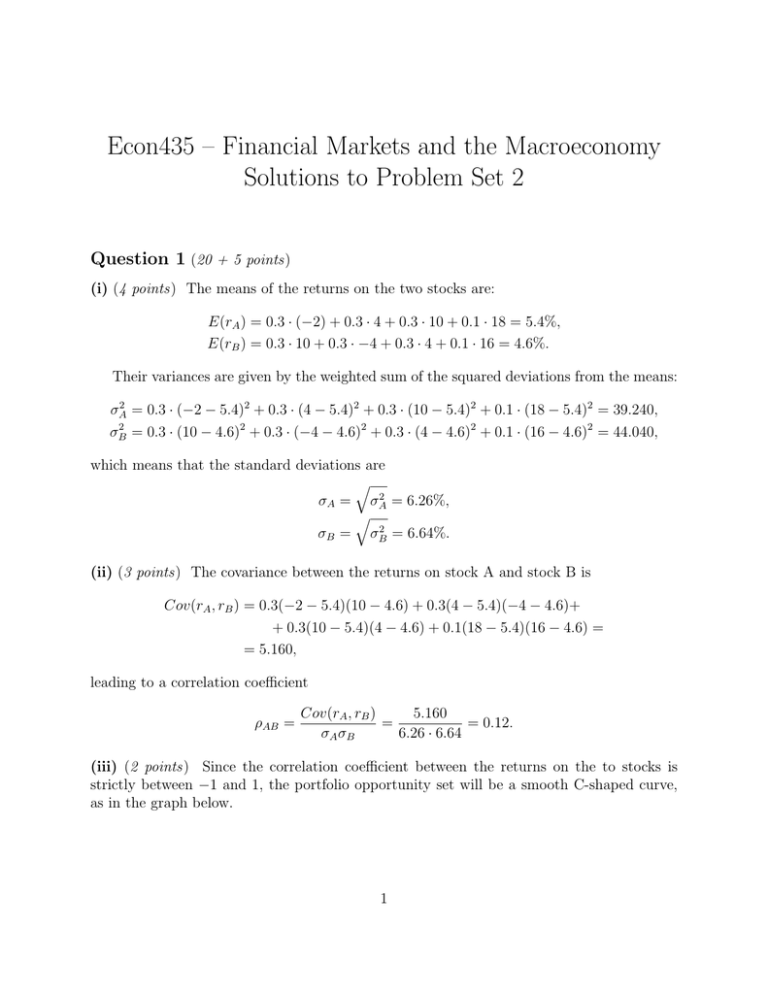
Econ435 – Financial Markets and the Macroeconomy
Solutions to Problem Set 2
Question 1 (20 + 5 points)
(i) (4 points) The means of the returns on the two stocks are:
E(rA ) = 0.3 · (−2) + 0.3 · 4 + 0.3 · 10 + 0.1 · 18 = 5.4%,
E(rB ) = 0.3 · 10 + 0.3 · −4 + 0.3 · 4 + 0.1 · 16 = 4.6%.
Their variances are given by the weighted sum of the squared deviations from the means:
σA2 = 0.3 · (−2 − 5.4)2 + 0.3 · (4 − 5.4)2 + 0.3 · (10 − 5.4)2 + 0.1 · (18 − 5.4)2 = 39.240,
σB2 = 0.3 · (10 − 4.6)2 + 0.3 · (−4 − 4.6)2 + 0.3 · (4 − 4.6)2 + 0.1 · (16 − 4.6)2 = 44.040,
which means that the standard deviations are
q
σA = σA2 = 6.26%,
q
σB = σB2 = 6.64%.
(ii) (3 points) The covariance between the returns on stock A and stock B is
Cov(rA , rB ) = 0.3(−2 − 5.4)(10 − 4.6) + 0.3(4 − 5.4)(−4 − 4.6)+
+ 0.3(10 − 5.4)(4 − 4.6) + 0.1(18 − 5.4)(16 − 4.6) =
= 5.160,
leading to a correlation coefficient
ρAB =
Cov(rA , rB )
5.160
=
= 0.12.
σA σB
6.26 · 6.64
(iii) (2 points) Since the correlation coefficient between the returns on the to stocks is
strictly between −1 and 1, the portfolio opportunity set will be a smooth C-shaped curve,
as in the graph below.
1
Figure 1: Portfolio Opportunity Set.
(iv) (8 points) In order to calculate the optimal proportions to be invested in the risky
portfolio and in the risk-free free asset, we first need to find the mean and variance of the
risky portfolio. They are:
E(rp ) = wA E(rA ) + wB E(rB ) = 0.78 · 5.4% + 0.22 · 4.6% = 5.22%,
2 2
2 2
σp2 = wA
σA + wB
σB + 2wA wB Cov(rA , rB )
= 0.782 · 39.240 + 0.222 · 44.040 + 2 · 0.78 · 0.22 · 5.160
= 27.78,
q
σp = σp2 = 5.27%.
Note that by combining stock A and stock B, investor X obtained a portfolio with lower
risk than both A and B, but with a higher return than stock B.
Using this information, we can now calculate the optimal proportion to be invested in
the risky portfolio:
y∗ =
E(rp ) − rf
5.22 − 4
=
= 0.73.
2
0.01Aσp
0.01 · 6 · 27.78
2
The proportion to be invested in the risk-free asset is 1 − y ∗ = 0.27. This enables us to
calculate the mean, variance and standard deviation of the complete portfolio:
E(rC ) = y ∗ E(rp ) + (1 − y ∗ )rf = 0.73 · 5.22% + 0.27 · 4% = 4.9%,
σC2 = y ∗2 σp2 = 0.732 · 27.78 = 14.98,
q
σC = σC2 = 3.87%.
Graphically, we can represent this as in the next figure.
Figure 2: Optimal Complete Portfolio.
(v) (3 points) If the borrowing rate is higher than the lending rate, then the CAL would
have a “kink” like in the graph below (either of the explanations was considered correct).
Since investor X is not a borrower, the optimal complete portfolio would not change. It
would still lie on the “original” Capital Allocation Line and would not be affected by the
higher borrowing interest rate.
(vi) (extra credit – 5 points) Any rational investor will choose the risk-free asset with the
highest rate of return. Again, it is important that investor X is not a borrower. In this case,
the original risk-free rate offers the highest rate of return (as compared to the new risk-free
3
Figure 3: Optimal Complete Portfolio with Higher Borrowing Rate.
asset). Hence, investor X will choose the same risk-free asset and thus end up with the same
optimal complete portfolio as before. In conclusion, nothing changes.
The situation would be different if investor X were a borrower. In this case, the new
risk-free asset brings a lower interest on borrowing, and thus the investor would prefer it to
the original risk-free asset. The optimal complete portfolio would change (you would need
to redo the calculations in part iv, using the new risk-free rate instead of the old one) and
investor X would end up borrowing even more.
4