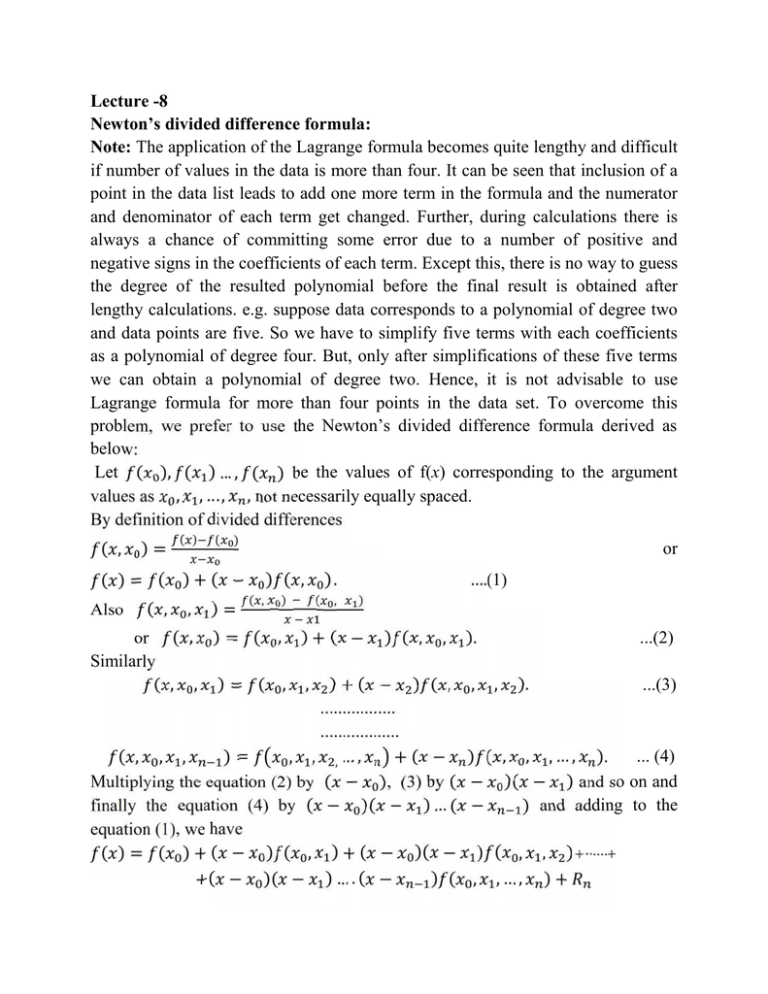
Lecture -8
Newton’s divided difference formula:
Note: The application of the Lagrange formula becomes quite lengthy and difficult
if number of values in the data is more than four. It can be seen that inclusion of a
point in the data list leads to add one more term in the formula and the numerator
and denominator of each term get changed. Further, during calculations there is
always a chance of committing some error due to a number of positive and
negative signs in the coefficients of each term. Except this, there is no way to guess
the degree of the resulted polynomial before the final result is obtained after
lengthy calculations. e.g. suppose data corresponds to a polynomial of degree two
and data points are five. So we have to simplify five terms with each coefficients
as a polynomial of degree four. But, only after simplifications of these five terms
we can obtain a polynomial of degree two. Hence, it is not advisable to use
Lagrange formula for more than four points in the data set. To overcome this
problem, we prefer to use the Newton’s divided difference formula derived as
below:
Let ( ), ( ) … , ( ) be the values of f(x) corresponding to the argument
values as , , … , , not necessarily equally spaced.
By definition of divided differences
( ,
)=
( )
(
)
( )= ( )+( −
Also
( ,
,
)=
or
( ,
) ( ,
)
(
).
,
)
or ( , ) = ( , ) + ( − ) ( , ,
Similarly
( , , )= ( , , )+( − ) ( ,
.................
..................
( , , ,
)=
, , ,…,
+( −
Multiplying the equation (2) by ( − ), (3) by (
finally the equation (4) by ( − )( − ) … (
equation (1), we have
( ) = ( ) + ( − ) ( , ) + ( − )( −
) (
+( − )( − ) … . ( −
….(1)
).
,
...(2)
,
).
...(3)
) ( , , , … , ).
... (4)
− )( − ) and so on and
−
) and adding to the
) ( ,
, ,…,
, )  ......
)+
where the remainder
is given by
= ( − )( − ) ...... ( − ) ( , , , … ).
Assuming that ( )is a polynomial of degree n, ( , , , … , ) vanishes being
(n+1) th -order divided difference, so that
( ) = ( ) + ( − ) ( , ) + ( − )( − ) ( , , ) ...... 
) ( , , , … , ).
+( − )( − ) … ( −
......(5)
This is called Newton’s divided difference Formula of Interpolation.
Note: As Newton’s divided difference formula requires the divided difference
table, it will be better if we rearrange the values of argument before preparing the
table either in ascending or descending order. If will be helpful in preparing the
table. Formula shows that it uses only the leading differences of various orders. So,
once the table is prepared, it is very easy to use. Also, if any order differences are
zeros, then one can predict the degree of interpolated polynomial from the table
without any calculation.
Example : Find the polynomial of the lowest possible degree which assumes the
values 3, 12, 15, -21 when x has the values 3, 2, 1, -1, respectively. Hence find
f(0).
Solution : Divided difference table
( )
∆ ( )
-1
-21
+18
1
15
-3
2
12
-9
3
3
∆
( )
∆
-7
1
-3
Using Newton’s divided difference formula, we get
( ) = −21 + − (−1)  18 + ( + 1)( − 1)  (−7)
+ ( + 1)( − 1)( − 2)  1
= −21 + 18( + 1) + ( − 1)(−7) + ( − 2 − + 2)
f (x) = x3 - 9 x2 + 17 x + 6. Hence f (0) = 6.
Example : The observed values of a function are respectively 168, 120, 72 and 63
at the four positions 3, 7, 9 and 10 of the independent variable. What is the best
estimated value of the function at the position 6 of the independent variable?
Solution : The divided difference table is given as follows :
( )
∆ ( )
∆ ( )
3
168
7
120
9
72
10
63
Hence
120 − 168
= −12
7−3
72 − 120
= −24
9−7
−24 + 12
= −2
9−3
63 − 72
= −9
10 − 9
−9 + 24
=5
10 − 7
∆
( )
5 − (−2)
=1
10 − 3
f  x   f  x0    x  x0  f  x0 , x1    x  x0  x  x1  f  x0 , x1 , x2 
  x  x0  x  x1  x  x2  f  x0 , x1 , x2 , x3 
= 168 + ( − 3)(−12) + ( − 3)( − 7)(−2) + ( − 3)( − 7)( − 9)(1)
=
− 21 + 119 − 27.
When = 6, the estimated value of the function is given by
(6) = 6 − 21 × 6 + 119 × 6 − 27 = 147