Natural Language Processing
Parts of Speech
Part‐of‐Speech Tagging
Dan Klein – UC Berkeley
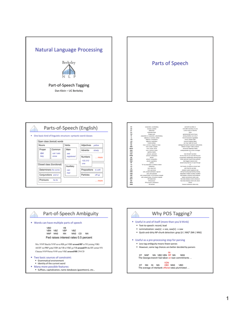
Parts‐of‐Speech (English)
 One basic kind of linguistic structure: syntactic word classes
Open class (lexical) words
Nouns
Verbs
Proper
Common
IBM
Italy
Main
cat / cats
snow
see
registered
yellow
Adverbs
slowly
Numbers
… more
122,312
one
Closed class (functional)
Auxiliary
Determiners the some
Prepositions to with
can
had
Conjunctions and or
Pronouns
Adjectives
Particles
he its
off up
… more
Part‐of‐Speech Ambiguity
VBZ
NNS
VB
VBP
NN
VBZ
NNS
CD
conjunction, coordinating
and both but either or
CD
DT
numeral, cardinal
determiner
mid-1890 nine-thirty 0.5 one
a all an every no that the
EX
FW
existential there
foreign word
there
gemeinschaft hund ich jeux
IN
JJ
JJR
preposition or conjunction, subordinating
adjective or numeral, ordinal
adjective, comparative
among whether out on by if
third ill-mannered regrettable
braver cheaper taller
JJS
MD
adjective, superlative
modal auxiliary
bravest cheapest tallest
can may might will would
NN
NNP
NNPS
noun, common, singular or mass
noun, proper, singular
noun, proper, plural
cabbage thermostat investment subhumanity
Motown Cougar Yvette Liverpool
Americans Materials States
NNS
POS
noun, common, plural
genitive marker
undergraduates bric-a-brac averages
' 's
PRP
PRP$
RB
pronoun, personal
pronoun, possessive
adverb
hers himself it we them
her his mine my our ours their thy your
occasionally maddeningly adventurously
RBR
RBS
adverb, comparative
adverb, superlative
further gloomier heavier less-perfectly
best biggest nearest worst
RP
TO
UH
particle
"to" as preposition or infinitive marker
interjection
aboard away back by on open through
to
huh howdy uh whammo shucks heck
VB
VBD
verb, base form
verb, past tense
ask bring fire see take
pleaded swiped registered saw
VBG
VBN
verb, present participle or gerund
verb, past participle
stirring focusing approaching erasing
dilapidated imitated reunifed unsettled
VBP
VBZ
WDT
verb, present tense, not 3rd person singular
verb, present tense, 3rd person singular
WH-determiner
twist appear comprise mold postpone
bases reconstructs marks uses
that what whatever which whichever
WP
WP$
WH-pronoun
WH-pronoun, possessive
that what whatever which who whom
whose
WRB
Wh-adverb
however whenever where why
Why POS Tagging?
 Useful in and of itself (more than you’d think)
 Words can have multiple parts of speech
VBD
VBN
NNP
CC
NN
Fed raises interest rates 0.5 percent
 Text‐to‐speech: record, lead
 Lemmatization: saw[v]  see, saw[n]  saw
 Quick‐and‐dirty NP‐chunk detection: grep {JJ | NN}* {NN | NNS}
 Useful as a pre‐processing step for parsing
 Less tag ambiguity means fewer parses
 However, some tag choices are better decided by parsers
 Two basic sources of constraint:
 Grammatical environment
 Identity of the current word
 Many more possible features:
 Suffixes, capitalization, name databases (gazetteers), etc…
IN
DT NNP
NN VBD VBN RP NN
NNS
The Georgia branch had taken on loan commitments …
VDN
DT NN IN NN
VBD NNS
VBD
The average of interbank offered rates plummeted …
1
Classic Solution: HMMs

We want a model of sequences s and observations w
s0
Part‐of‐Speech Tagging

s1
s2
sn
w1
w2
wn
Assumptions:





States are tag n‐grams
Usually a dedicated start and end state / word
Tag/state sequence is generated by a markov model
Words are chosen independently, conditioned only on the tag/state
These are totally broken assumptions: why?
States
Estimating Transitions
 States encode what is relevant about the past
 Transitions P(s|s’) encode well‐formed tag sequences
 In a bigram tagger, states = tags
 Use standard smoothing methods to estimate transitions:
P(ti | ti 1 , ti 2 )  2 Pˆ (ti | ti 1 , ti 2 )  1Pˆ (ti | ti 1 )  (1  1  2 ) Pˆ (ti )
<>
< t1>
< t2>
< tn>
s0
s1
s2
sn
 Can get a lot fancier (e.g. KN smoothing) or use higher orders, but in this case it doesn’t buy much
w1
w2
wn
 One option: encode more into the state, e.g. whether the previous word was capitalized (Brants 00)
 In a trigram tagger, states = tag pairs
<,>
< , t1>
< t1, t2>
s0
s1
s2
sn
w1
w2
wn
< tn-1, tn>
 BIG IDEA: The basic approach of state‐splitting / refinement turns out to be very important in a range of tasks
Estimating Emissions
Disambiguation (Inference)
 Problem: find the most likely (Viterbi) sequence under the model
 Emissions are trickier:




Words we’ve never seen before
Words which occur with tags we’ve never seen them with
One option: break out the fancy smoothing (e.g. KN, Good‐Turing)
Issue: unknown words aren’t black boxes:
343,127.23
11-year
Minteria
reintroducibly
 Basic solution: unknown words classes (affixes or shapes)
D+,D+.D+
D+-x+
Xx+
x+-“ly”
 Common approach: Estimate P(t|w) and invert
 [Brants 00] used a suffix trie as its (inverted) emission model
 Given model parameters, we can score any tag sequence
<,>
<,NNP>
<NNP, VBZ>
NNP
VBZ
Fed
raises
<VBZ, NN>
<NN, NNS> <NNS, CD>
NN
NNS
interest rates
<CD, NN>
<STOP>
CD
NN
.
0.5
percent
.
P(NNP|<,>) P(Fed|NNP) P(VBZ|<NNP,>) P(raises|VBZ) P(NN|VBZ,NNP)…..
 In principle, we’re done – list all possible tag sequences, score each one, pick the best one (the Viterbi state sequence) NNP VBZ NN NNS CD NN
logP = -23
NNP NNS NN NNS CD NN
logP = -29
NNP VBZ VB NNS CD NN
logP = -27
2
The State Lattice / Trellis
The State Lattice / Trellis
^
^
^
^
^
^
^
^
^
^
^
^
N
N
N
N
N
N
N
N
N
N
N
N
V
V
V
V
V
V
V
V
V
V
V
V
J
J
J
J
J
J
J
J
J
J
J
J
D
D
D
D
D
D
D
D
D
D
D
D
$
$
$
$
$
$
$
$
$
$
$
$
Fed
raises
interest
rates
END
Fed
raises
interest
rates
END
START
START
So How Well Does It Work?
Overview: Accuracies
 Roadmap of (known / unknown) accuracies:
 Choose the most common tag
 90.3% with a bad unknown word model
 93.7% with a good one
 TnT (Brants, 2000):
 A carefully smoothed trigram tagger
 Suffix trees for emissions
 96.7% on WSJ text (SOA is ~97.5%)
JJ
JJ
NN
chief executive officer
 Noise in the data
NN
JJ
NN
chief executive officer
 Many errors in the training and test corpora
JJ
NN
NN
chief executive officer
NN
NN
NN
chief executive officer
DT NN IN NN
VBD NNS
VBD
The average of interbank offered rates plummeted …
 Probably about 2% guaranteed error
from noise (on this data)
 Most freq tag: ~90% / ~50%
 Trigram HMM: ~95% / ~55%
 TnT (HMM++): 96.2% / 86.0%




93.7% / 82.6%
96.9% / 86.9%
97+% / 89+%
~98%
Maxent P(t|w): MEMM tagger: State‐of‐the‐art: Upper bound: Most errors
on unknown
words
Common Errors
 Common errors [from Toutanova & Manning 00]
Richer Features
NN/JJ
NN
official knowledge
VBD RP/IN DT NN
made up the story
RB VBD/VBN NNS
recently sold shares
3
Better Features
Why Linear Context is Useful
 Lots of rich local information!
 Can do surprisingly well just looking at a word by itself:






Word
Lowercased word
Prefixes
Suffixes
Capitalization
Word shapes
RB
PRP VBD IN RB IN PRP VBD .
They left as soon as he arrived .
the: the  DT
Importantly: importantly  RB
unfathomable: un‐  JJ
Surprisingly: ‐ly  RB
Meridian: CAP  NNP
35‐year: d‐x  JJ
 Then build a maxent (or whatever) model to predict tag
 Maxent P(t|w): 93.7% / 82.6%
 We could fix this with a feature that looked at the next word
JJ
NNP NNS VBD
VBN
.
Intrinsic flaws remained undetected .
 We could fix this by linking capitalized words to their lowercase versions
 Solution: discriminative sequence models (MEMMs, CRFs)
s3
 Reality check:
 Taggers are already pretty good on WSJ journal text…
 What the world needs is taggers that work on other text!
 Though: other tasks like IE have used the same methods to good effect
w3
Sequence‐Free Tagging?
 What about looking at a word and its environment, but no sequence information?






Add in previous / next word the __
Previous / next word shapes
X __ X
Occurrence pattern features
[X: x X occurs]
Crude entity detection
__ ….. (Inc.|Co.)
Phrasal verb in sentence? put …… __
Conjunctions of these things
Feature‐Rich Sequence Models
 Problem: HMMs make it hard to work with arbitrary features of a sentence
t3
w2
w3
w4
 Example: name entity recognition (NER)
PER PER O
O
O
O
ORG
O
Prev
Cur
Next
State
Other
???
???
Word
at
Grace Road
Tag
IN
NNP
NNP
Sig
x
Xx
Xx
MEMM Taggers
 Train up P(ti|w,ti‐1,ti‐2) as a normal maxent model, then use to score sequences
 This is referred to as an MEMM tagger [Ratnaparkhi 96]
 Beam search effective! (Why?)
 What about beam size 1?
O
O
O
O O LOC LOC O
Local Context
 All features except sequence: 96.6% / 86.8%
 Uses lots of features: > 200K
 Why isn’t this the standard approach?
 Idea: left‐to‐right local decisions, condition on previous tags and also entire input
O
Tim Boon has signed a contract extension with Leicestershire which will keep him at Grace Road .
NER Features
Feature Weights
Because of regularization
term, the more common
prefixes have larger
weights even though
entire-word features are
more specific.
Local Context
Feature Type
Feature
PERS
LOC
Previous word
at
-0.73
0.94
Current word
Grace
0.03
0.00
<G
0.45
-0.04
Beginning bigram
Current POS tag
NNP
0.47
0.45
Prev and cur tags
IN NNP
-0.10
0.14
Other
-0.70
-0.92
Prev
Cur
Next
Previous state
Current signature
Xx
0.80
0.46
State
Other
???
???
Prev state, cur sig
O-Xx
0.68
0.37
Word
at
Grace Road
Prev-cur-next sig
x-Xx-Xx
-0.69
0.37
Tag
IN
NNP
NNP
P. state - p-cur sig
O-x-Xx
-0.20
0.82
Sig
x
Xx
Xx
-0.58
2.68
…
Total:
4
Perceptron Taggers
[Collins 01]
 Linear models:
Conditional Random Fields (and Friends)
 … that decompose along the sequence
 … allow us to predict with the Viterbi algorithm
 … which means we can train with the perceptron algorithm (or related updates, like MIRA)
Conditional Random Fields
 Make a maxent model over entire taggings
CRFs
 Like any maxent model, derivative is:
 MEMM
 So all we need is to be able to compute the expectation of each feature (for example the number of times the label pair DT‐NN occurs, or the number of times NN‐interest occurs) under the model distribution
 CRF
 Critical quantity: counts of posterior marginals: Computing Posterior Marginals
 How many (expected) times is word w tagged with s?
Transformation‐Based Learning
 [Brill 95] presents a transformation‐based tagger
 Label the training set with most frequent tags
DT MD VBD VBD .
The can was rusted .
 How to compute that marginal?
^
^
^
^
^
^
N
N
N
N
N
N
V
V
V
V
V
V
J
J
J
J
J
J
D
D
D
D
D
D
$
START
$
$
$
$
Fed
raises
interest
rates
$
END
 Add transformation rules which reduce training mistakes
 MD  NN : DT __
 VBD  VBN : VBD __ .
 Stop when no transformations do sufficient good
 Does this remind anyone of anything?
 Probably the most widely used tagger (esp. outside NLP)
 … but definitely not the most accurate: 96.6% / 82.0 %
5
Learned Transformations
 What gets learned? [from Brill 95]
Domain Effects
 Accuracies degrade outside of domain
 Up to triple error rate
 Usually make the most errors on the things you care about in the domain (e.g. protein names)
 Open questions
 How to effectively exploit unlabeled data from a new domain (what could we gain?)
 How to best incorporate domain lexica in a principled way (e.g. UMLS specialist lexicon, ontologies)
Unsupervised Tagging?
 AKA part‐of‐speech induction
 Task:
Unsupervised Tagging
 Raw sentences in
 Tagged sentences out
 Obvious thing to do:
 Start with a (mostly) uniform HMM
 Run EM
 Inspect results
EM for HMMs: Process
 Alternate between recomputing distributions over hidden variables (the tags) and reestimating parameters
 Crucial step: we want to tally up how many (fractional) counts of each kind of transition and emission we have under current params:
Merialdo: Setup
 Some (discouraging) experiments [Merialdo 94]
 Setup:
 You know the set of allowable tags for each word
 Fix k training examples to their true labels
 Learn P(w|t) on these examples
 Learn P(t|t‐1,t‐2) on these examples
 On n examples, re‐estimate with EM
 Same quantities we needed to train a CRF!
 Note: we know allowed tags but not frequencies
6
Merialdo: Results
Distributional Clustering
 the president said that the downturn was over 
president
the __ of
president
the __ said
governor
the __ of
governor
the __ appointed
said
sources __ 
said
president __ that
reported
sources __ 
president
governor
the
a
said
reported
[Finch and Chater 92, Shuetze 93, many others]
Distributional Clustering
Nearest Neighbors
 Three main variants on the same idea:
 Pairwise similarities and heuristic clustering
 E.g. [Finch and Chater 92]
 Produces dendrograms
 Vector space methods
 E.g. [Shuetze 93]
 Models of ambiguity
 Probabilistic methods
 Various formulations, e.g. [Lee and Pereira 99]
Dendrograms _
A Probabilistic Version?
P ( S , C )   P (ci ) P ( wi | ci ) P ( wi 1 , wi 1 | ci )
i
c1
c2
c3
c4 c5
c6
c7
c8
 the president said that the downturn was over 
P( S , C )   P ( wi | ci ) P (ci | ci 1 )
i
c1
c2
c3
c4 c5
c6
c7
c8
 the president said that the downturn was over 
7