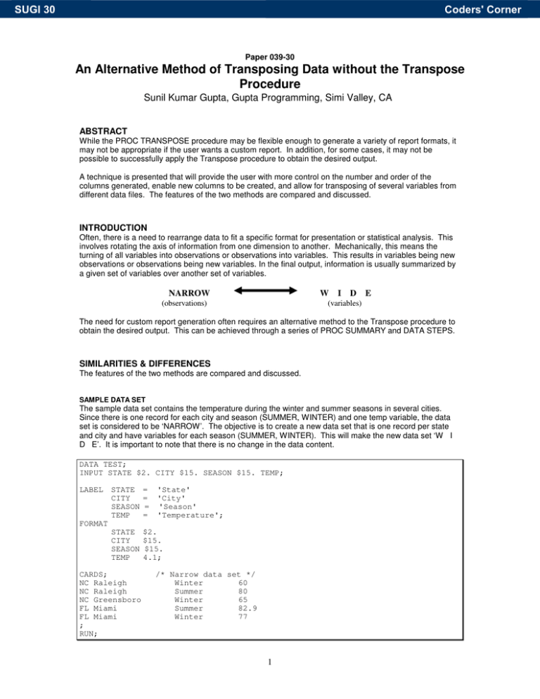
SUGI 30
Coders' Corner
Paper 039-30
An Alternative Method of Transposing Data without the Transpose
Procedure
Sunil Kumar Gupta, Gupta Programming, Simi Valley, CA
ABSTRACT
While the PROC TRANSPOSE procedure may be flexible enough to generate a variety of report formats, it
may not be appropriate if the user wants a custom report. In addition, for some cases, it may not be
possible to successfully apply the Transpose procedure to obtain the desired output.
A technique is presented that will provide the user with more control on the number and order of the
columns generated, enable new columns to be created, and allow for transposing of several variables from
different data files. The features of the two methods are compared and discussed.
INTRODUCTION
Often, there is a need to rearrange data to fit a specific format for presentation or statistical analysis. This
involves rotating the axis of information from one dimension to another. Mechanically, this means the
turning of all variables into observations or observations into variables. This results in variables being new
observations or observations being new variables. In the final output, information is usually summarized by
a given set of variables over another set of variables.
NARROW
W
(observations)
I
D
(variables)
E
The need for custom report generation often requires an alternative method to the Transpose procedure to
obtain the desired output. This can be achieved through a series of PROC SUMMARY and DATA STEPS.
SIMILARITIES & DIFFERENCES
The features of the two methods are compared and discussed.
SAMPLE DATA SET
The sample data set contains the temperature during the winter and summer seasons in several cities.
Since there is one record for each city and season (SUMMER, WINTER) and one temp variable, the data
set is considered to be ‘NARROW’. The objective is to create a new data set that is one record per state
and city and have variables for each season (SUMMER, WINTER). This will make the new data set ‘W I
D E’. It is important to note that there is no change in the data content.
DATA TEST;
INPUT STATE $2. CITY $15. SEASON $15. TEMP;
LABEL
STATE
CITY
SEASON
TEMP
=
=
=
=
'State'
'City'
'Season'
'Temperature';
STATE
CITY
SEASON
TEMP
$2.
$15.
$15.
4.1;
FORMAT
CARDS;
NC Raleigh
NC Raleigh
NC Greensboro
FL Miami
FL Miami
;
RUN;
/* Narrow data set */
Winter
60
Summer
80
Winter
65
Summer
82.9
Winter
77
1
SUGI 30
Coders' Corner
PROC TRANSPOSE
The Transpose procedure assumes the data to be summarized by the grouping set of variables.
1. Sort by the grouping variables STATE and CITY. These variables will be summarized in the report.
PROC SORT DATA=TEST;
BY STATE CITY;
RUN;
2. Apply the Transpose procedure. This rotates the data.
The OUT option allows for saving of the results into a data set. The BY statement identifies the grouping
variables STATE and CITY. These grouping variables are not transposed. The ID statement identifies the
variable SEASON to represent the new variables in the transposed data set. The VAR statement identifies
the measuring variable that will be transposed and saved in the new variables based on the SEASON’s
value. A format statement can be applied to the measuring variable.
PROC TRANSPOSE DATA=TEST OUT=TRANS_DS (DROP = _NAME_ _LABEL_);
BY STATE CITY;
ID SEASON;
VAR TEMP;
FORMAT TEMP 4.1;
RUN;
The final data set is sorted by STATE and CITY and has variables SUMMER and WINTER with the TEMP
values. Note that five observations from the ‘NARROW’ data set TEST were converted to three
observations in the ‘W I D E’ data set TRANS_DS.
Output - TRANS_DS data set
Obs
1
2
3
STATE
FL
NC
NC
CITY
Miami
Greensboro
Raleigh
/* W I D E data set */
Summer
Winter
82.9
.
80.0
77.0
65.0
60.0
ALTERNATIVE METHOD TO PROC TRANSPOSE
This method consists of a series of PROC SUMMARY and DATA STEPS to achieve the reporting data set.
The following 6 steps are followed:
1. Summarize the measuring variable by the grouping variables STATE and CITY.
2. Create column variables in the master data set and initialize them to zero.
3. Summarize by the grouping variables STATE, CITY, and SEASON.
4. Rename grouping variables in the second data set.
5. Construct nested do-loops to store the measuring variable for matching group variables.
6. Select only one record for grouping variables STATE and CITY.
1. Summarize the measuring variable by the grouping variables STATE and CITY. This will formulate the
master reporting data set TEST1 to be one record per state and city. You can also drop the TEMP variable.
PROC SUMMARY DATA=TEST NWAY MISSING;
CLASS STATE CITY;
VAR TEMP;
OUTPUT OUT=TEST1 (DROP=_TYPE_ _FREQ_ TEMP) SUM=;
RUN;
2
SUGI 30
Coders' Corner
Output – TEST1 data set (One record per state and city)
Obs
1
2
3
STATE
FL
NC
NC
CITY
Miami
Greensboro
Raleigh
2. Based on each unique value of the SEASON variable, create that variable in the master data set and
initialize the values to missing. These variables will store the summarized measuring variables for the
report layout.
DATA TESTM1;
SET TEST1;
SUMMER=. ;
WINTER=. ;
RUN;
Output – TESTM1 data set
Obs
1
2
3
STATE
FL
NC
NC
CITY
Miami
Greensboro
Raleigh
SUMMER
WINTER
.
.
.
.
.
.
3. Summarize by the grouping variables STATE, CITY, and SEASON. Depending on what type of data is
collected, the MEAN= option may be more appropriate for calculating an average value as compared to the
summation of the values. This will summarize the measuring variable by all the possible combinations of
the analysis variables STATE, CITY and SEASON. This makes the TEST2 data set one record per state,
city and season.
PROC SUMMARY DATA=TEST NWAY MISSING;
CLASS STATE CITY SEASON;
VAR TEMP;
OUTPUT OUT=TEST2 (DROP=_TYPE_ _FREQ_) SUM=;
RUN;
Output – TEST2 data set (One record per state, city and season)
Obs
1
2
3
4
5
STATE
FL
FL
NC
NC
NC
CITY
SEASON
TEMP
Miami
Miami
Greensboro
Raleigh
Raleigh
Summer
Winter
Winter
Summer
Winter
82.9
77.0
65.0
80.0
60.0
4. Rename the grouping variables in the second summarized data set TEST2. This will allow for easier
identification of the source of the common variables STATE and CITY. This step is needed to allow the
matching of the grouping variables when the two data sets TESTM1 and TEST2R are combined in the next
step.
DATA TEST2R;
SET TEST2;
RENAME STATE=STATE1;
RENAME CITY=CITY1;
RUN;
3
SUGI 30
Coders' Corner
Output – TEST2R data set
Obs
STATE1
1
2
3
4
5
FL
FL
NC
NC
NC
CITY1
SEASON
TEMP
Miami
Miami
Greensboro
Raleigh
Raleigh
Summer
Winter
Winter
Summer
Winter
82.9
77.0
65.0
80.0
60.0
5. Construct nested do-loops to store the measuring variable TEMP in variables SUMMER and WINTER for
matching group variables STATE and CITY. For each record in the TESTM1 data set, process all records
in the TEST2R data set. When the variable STATE matches STATE1 and CITY matches CITY1, then the
value of TEMP variable is assigned. An OUTPUT statement is then executed to create the record. At the
end of the outer do loop, a STOP statement is required to exit the data step.
Since this data step has two SET statements, SAS does not initialize the variables SUMMER and WINTER
to missing for each iteration of the TEST2R data set. In fact, the values are retained until the next record in
the TESTM1 data set is processed. This step rearranges the TEST2R data set’s orientation from variables
to observations.
DATA TESTM2;
PUT @1 'START 1';
OBSNUM=1;
DO OBSNUM=1 TO LASTR2;
SET TESTM1 POINT=OBSNUM NOBS=LASTR2;
OBS=1;
DO OBS=1 TO LASTR;
SET TEST2R POINT=OBS NOBS=LASTR;
IF STATE=STATE1 AND CITY=CITY1 THEN DO;
IF SEASON='Summer' THEN SUMMER=TEMP;
IF SEASON='Winter' THEN WINTER=TEMP;
OUTPUT;
END;
END;
END;
STOP;
RUN;
Note: For additional measuring variables, more conditional statements are needed to store the information
in the new column variables.
Output – TESTM2 data set (One record per state, city and season with summer and winter variables)
Obs STATE CITY
1
2
3
4
5
FL
FL
NC
NC
NC
Miami
Miami
Greensboro
Raleigh
Raleigh
SUMMER
WINTER
STATE1
82.9
82.9
.
80.0
80.0
.
77
65
.
60
FL
FL
NC
NC
NC
CITY1
SEASON
TEMP
Miami
Miami
Greensboro
Raleigh
Raleigh
Summer
Winter
Winter
Summer
Winter
82.9
77.0
65.0
80.0
60.0
6. Select only one record for grouping variables STATE and CITY. Because of the OUTPUT statement,
multiple records can be generated for the grouping variable. As a result, the data set needs to be indexed
by the grouping variables and only a single copy of the record should be stored in the resulting data set.
This constitutes the final reporting data set. The following unnecessary variables STATE1, CITY1,
SEASON and TEMP can be dropped in the final data set TESTM3.
4
SUGI 30
Coders' Corner
DATA TESTM3;
SET TESTM2;
BY STATE CITY;
IF LAST.CITY;
DROP STATE1 CITY1 SEASON TEMP;
RUN;
As you can see, the final data set is sorted by STATE and CITY and has variables SUMMER and WINTER
with the TEMP values. As with the Transpose procedure, the five observations from the ‘NARROW’ data
set TEST were converted to three observations in the ‘W I D E’ data set TESTM3.
Output – TESTM3 data set
Obs
1
2
3
STATE
FL
NC
NC
CITY
Miami
Greensboro
Raleigh
/* W I D E data set */
Summer
Winter
82.9
.
80.0
77.0
65.0
60.0
ADVANTAGES
A variety of reports can be generated with the proposed alternative method. Several advantages using the
alternative method were found.
•
It allows for greater control on the number of columns in the report. New columns can be created. In
addition, the order of columns can be specified. Unwanted columns can be removed.
•
It is a valid method for custom reports requiring the transposing of several variables from different data
files.
•
It allows for the addition of a percent column in the report.
DISADVANTAGES
There are several disadvantages to the alternative method.
•
The proposed method requires a greater understanding of the DATA STEP. It also requires a solid
understanding of PROC SUMMARY. In addition, it may take a longer time to write the program.
•
The proposed alternative to the Transpose Procedure works best for a specified number of columns in
the report. This is because a field must be defined for each case of the transposed variable.
Therefore, if the ID variable contains many types of cases, then the Transpose Procedure is a better
choice because it automatically accounts for this. The Transpose Procedure automatically creates a
column for each case.
SUMMARY
The SAS programmer has a variety of tools available to complete a reporting objective. The need may
arise to become creative in solving reporting obstacles. As often is the case, there is more than one way to
achieve an outcome.
REFERENCES
Turning a ‘Wide’ Data Set into a ‘Narrow’ Data Set, The TRANSPOSE Procedure (also known as ‘The Easy
Way’), Technical Tips: SAS Bits and Bytes, Melinda Thielbar,
http://support.sas.com/sassamples/bitandbytes/transpose2.html
Turning a ‘Wide’ Data Set into a ‘Narrow’ Data Set, Using a DATA Step (also known as ‘The Hard Way’),
Technical Tips: SAS Bits and Bytes, Melinda Thielbar,
http://support.sas.com/sassamples/bitandbytes/transpose1.html
5
SUGI 30
Coders' Corner
SAS Procedures Guide, ver. 6, third edition.
TRADEMARK INFORMATION
SAS and all other SAS Institute Inc. product or service names are registered trademarks or trademarks of
SAS Institute Inc. in the USA and other countries. ® indicates USA registration.
ABOUT THE AUTHOR
The author welcomes your comments and suggestions on other methods of transposing data.
Sunil Gupta
Gupta Programming
213 Goldenwood Circle
Simi Valley, CA 93065-6772
(805) 584-6182
Sunil@GuptaProgramming.com
http://www.GuptaProgramming.com
Sunil is the principal consultant at Gupta Programming. He has been using SAS® software for over 13
years and is a SAS Base Certified Professional. He has participated in over 6 successful FDA
submissions. He is also the author of Quick Results with the Output Delivery System, developer of over five
SAS programming classes, developer of Clinical Trial Reporting Templates for quick generation of tables,
lists and graphs and was a SAS Institute Quality Partner™ for over 5 years. Currently, he is writing a new
book on Analysis and Reporting Made Easier Using SAS Learning Edition and is coauthoring the book,
Sharpening Your SAS Skills, to help users better understand and analyze the SAS programming language.
ACKNOWLEDGMENTS
The author would like to thank Dr. Fred Hoehler of Data Management Center, Santa Ana, CA and Kirk Paul
Lafler of Software Intelligence Corporation, Spring Valley, CA for their invaluable assistance in the
preparation of this paper.
6