Title
stata.com
graph twoway function — Twoway line plot of function
Syntax
Remarks and examples
Menu
Reference
Description
Also see
Options
Syntax
twoway function
y = f (x) if
in
, options
options
Description
range(# #)
range(varname)
n(#)
plot over x = # to #
plot over x = min to max of varname
evaluate at # points; default is 300
droplines(numlist)
base(#)
draw lines to axis at specified x values
base value for dropline(); default is 0
horizontal
draw plot horizontally
yvarformat(% fmt)
xvarformat(% fmt)
display format for y
display format for x
cline options
change look of plotted line
axis choice options
associate plot with alternative axis
twoway options
titles, legends, axes, added lines and text, by, regions, name,
aspect ratio, etc.
See [G-3] cline options, [G-3] axis choice options, and [G-3] twoway options.
All explicit options are rightmost, except horizontal, which is unique; see
[G-4] concept: repeated options.
if exp and in range play no role unless option range(varname) is specified.
In the above syntax diagram, f (x) stands for an expression in terms of x.
Menu
Graphics
>
Twoway graph (scatter, line, etc.)
Description
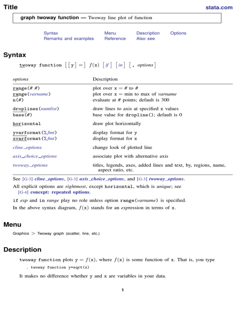
twoway function plots y = f (x), where f (x) is some function of x. That is, you type
. twoway function y=sqrt(x)
It makes no difference whether y and x are variables in your data.
1
2
graph twoway function — Twoway line plot of function
Options
range(# #) and range(varname) specify the range of values for x. In the first syntax, range() is
a pair of numbers identifying the minimum and maximum. In the second syntax, range() is a
variable name, and the range used will be obtained from the minimum and maximum values of
the variable. If range() is not specified, range(0 1) is assumed.
n(#) specifies the number of points at which f (x) is to be evaluated. The default is n(300).
droplines(numlist) adds dropped lines from the function down to, or up to, the axis (or y = base()
if base() is specified) at each x value specified in numlist.
base(#) specifies the base for the droplines(). The default is base(0). This option does not affect
the range of the axes, so you may also want to specify the axis scale option yscale(range(#))
as well; see [G-3] axis scale options.
horizontal specifies that the roles of y and x be interchanged and that the graph be plotted
horizontally rather than vertically (that the plotted function be reflected along the identity line).
yvarformat(% fmt) and xvarformat(% fmt) specify the display format to be used for y and x.
These formats are used when labeling the axes; see [G-3] axis label options.
cline options specify how the function line is rendered; see [G-3] cline options.
axis choice options associate the plot with a particular y or x axis on the graph; see
[G-3] axis choice options.
twoway options are a set of common options supported by all twoway graphs. These options allow
you to title graphs, name graphs, control axes and legends, add lines and text, set aspect ratios,
create graphs over by() groups, and change some advanced settings. See [G-3] twoway options.
Remarks and examples
Remarks are presented under the following headings:
Typical use
Advanced use 1
Advanced use 2
stata.com
graph twoway function — Twoway line plot of function
3
Typical use
You wish to plot the function y = exp(−x/6)sin(x) over the range 0 to 4π :
−.5
0
y
.5
1
. twoway function y=exp(-x/6)*sin(x), range(0 12.57)
0
5
10
15
x
A better rendition of the graph above is
−.5
0
y
.5
1
. twoway function y=exp(-x/6)*sin(x), range(0 12.57)
yline(0, lstyle(foreground))
xlabel(0 3.14 "{&pi}" 6.28 "2{&pi}" 9.42 "3{&pi}" 12.57 "4{&pi}")
plotregion(style(none))
xsca(noline)
0
π
2π
x
3π
4π
yline(0, lstyle(foreground)) added a line at y = 0; lstyle(foreground) gave the line
the same style as used for the axes. See [G-3] added line options.
xlabel(0 3.14 "{&pi}" 6.28 "2{&pi}" 9.42 "3{&pi}" 12.57 "4{&pi}") labeled the x axis
with the numeric values given; see [G-3] axis label options.
4
graph twoway function — Twoway line plot of function
plotregion(style(none)) suppressed the border around the plot region; see [G-3] region options.
xsca(noline) suppressed the drawing of the x-axis line; see [G-3] axis scale options.
Advanced use 1
The following graph appears in many introductory textbooks:
. twoway
function y=normalden(x),
|| function y=normalden(x),
|| function y=normalden(x),
||,
plotregion(style(none))
ysca(off) xsca(noline)
legend(off)
xlabel(-4 "-4 sd" -3 "-3
1 "1 sd" 2 "2
, grid gmin gmax)
xtitle("")
−4 sd
−3 sd
−2 sd
range(-4 -1.96) color(gs12) recast(area)
range(1.96 4)
color(gs12) recast(area)
range(-4 4) lstyle(foreground)
sd" -2 "-2 sd" -1 "-1 sd" 0 "mean"
sd" 3 "3 sd" 4 "4 sd"
−1 sd
mean
1 sd
2 sd
3 sd
4 sd
We drew the graph in three parts: the shaded area on the left, the shaded area on the right, and
then the overall function. To obtain the shaded areas, we used the advanced option recast(area)
so that, rather than the function being plotted by graph twoway line, it was plotted by graph
twoway area; see [G-3] advanced options and [G-2] graph twoway area. Concerning the overall
function, we drew it last so that its darker foreground-colored line would not get covered up by the
shaded areas.
graph twoway function — Twoway line plot of function
5
Advanced use 2
function plots may be overlaid with other twoway plots. For instance, function is one way to
add y = x lines to a plot:
1000
1100
1200
1300
1400
. use http://www.stata-press.com/data/r13/sp500, clear
(S&P 500)
. scatter open close, msize(*.25) mcolor(*.6) ||
function y=x, range(close) yvarlab("y=x") clwidth(*1.5)
1000
1100
Opening price
1200
1300
1400
y=x
In the above, we specified the advanced option yvarlab("y=x") so that the variable label of y
would be treated as “y=x” in the construction of the legend; see [G-3] advanced options. We specified
msize(*.25) to make the marker symbols smaller, and we specified mcolor(*.6) to make them
dimmer; see [G-4] relativesize and [G-4] colorstyle.
Reference
Cox, N. J. 2004. Stata tip 15: Function graphs on the fly. Stata Journal 4: 488–489.
Also see
[G-2] graph twoway line — Twoway line plots