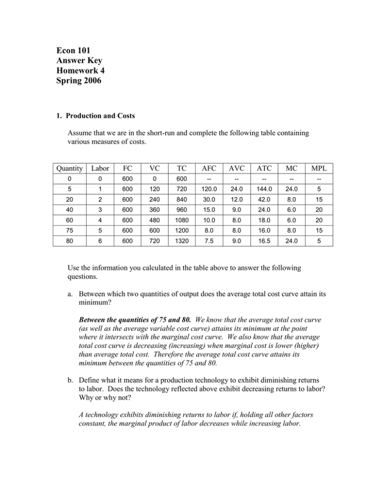
Econ 101
Answer Key
Homework 4
Spring 2006
1. Production and Costs
Assume that we are in the short-run and complete the following table containing
various measures of costs.
Quantity
Labor
FC
VC
TC
AFC
AVC
ATC
MC
MPL
0
0
600
0
600
--
--
--
--
--
5
1
600
120
720
120.0
24.0
144.0
24.0
5
20
2
600
240
840
30.0
12.0
42.0
8.0
15
40
3
600
360
960
15.0
9.0
24.0
6.0
20
60
4
600
480
1080
10.0
8.0
18.0
6.0
20
75
5
600
600
1200
8.0
8.0
16.0
8.0
15
80
6
600
720
1320
7.5
9.0
16.5
24.0
5
Use the information you calculated in the table above to answer the following
questions.
a. Between which two quantities of output does the average total cost curve attain its
minimum?
Between the quantities of 75 and 80. We know that the average total cost curve
(as well as the average variable cost curve) attains its minimum at the point
where it intersects with the marginal cost curve. We also know that the average
total cost curve is decreasing (increasing) when marginal cost is lower (higher)
than average total cost. Therefore the average total cost curve attains its
minimum between the quantities of 75 and 80.
b. Define what it means for a production technology to exhibit diminishing returns
to labor. Does the technology reflected above exhibit decreasing returns to labor?
Why or why not?
A technology exhibits diminishing returns to labor if, holding all other factors
constant, the marginal product of labor decreases while increasing labor.
Yes it does. At first, as the quantity of labor increases, the marginal product of
labor is increasing, but eventually towards the end of the table, the marginal
product of labor is decreasing as labor is increasing.
2. Perfect Competition
The market for gasoline in the City of Madison is characterized by perfect
competition. Firms and consumers are price takers and there is free entry and exit.
Assume this industry is a constant cost industry.
The total cost and marginal cost functions for an individual firm are given by the
following equations (assume all firms are identical in terms of their technologies, and
therefore their cost functions):
TC = (Qs)2 + 2*(Qs) + 9
MC = 2*Qs + 2
(Hint: You do not need the demand equation to solve parts a. and b.)
a. What is the equilibrium price that will prevail in the market?
P = 8. We know that firms always produce at the minimum of average total cost,
and we also know that average total cost attains its minimum when it intersects
marginal cost. Since TC and MC are given to us, we just need to construct ATC.
ATC = TC/Q = Qs + 2 + 9/Qs
Setting this equal to MC gives us: ATC = MC =
Qs + 2 + 9/Qs = 2*Qs + 2
9/Qs = Qs
9 = (Qs)2
Qs = 3.
Plugging Qs = 3 into either ATC or MC gives us that the price in the market is
P = 8.
b. What will be the output of each firm in the long-run equilibrium?
Qs = 3. In part a. we solved for the long-run equilibrium quantity of each firm.
Qs = 3.
Suppose that the aggregate demand is given by the following equation:
Demand: Pd = 500 – 2*Qd
c. How many firms will exist in the long-run equilibrium?
82 firms. We know that each firm will produce 3 units at a price of 8, so we need
to find out how many firms are needed to satisfy demand when price equals 8.
Plugging P = 8 into the demand equation gives us that the aggregate quantity
demanded equals 246.
P = 8 = 500 – 2*Qd
2*Qd = 500 – 8
2*Qd = 492
Qd = 246
Since each firm produces a quantity of 3 in the long-run equilibrium, then the
number of firms equals 246/3 = 82.
Number of firms * Quantity of each firm = Total Quantity
Number of firms = Total Quantity / Quantity of each firm
Number of firms = 246 / 3= 82.
Suppose that the City Council votes for an increase in the price of public
transportation such that the new aggregate demand curve for gasoline shifts out and is
given by the following equation:
Pd = 900 - 2*Qd
(Hint: Before diving into calculations think about the questions and about what you
know about perfect competition.)
d. Will the new short-run profits be negative, positive, or zero?
Positive. When demand shifts out (shifts to the right), we know that this is going
to lead to a higher equilibrium price and therefore positive profits in the shortrun.
e. Will the new long-run profits be negative, positive, or zero?
Zero. We know that under perfect competition long-run profits are zero.
So even though there are positive profits in the short-run, there will be entry to
the point where long-run profits are again zero.
f. What will be the new long-run equilibrium price?
P = 8. The long-run equilibrium price under perfect competition is always given
by the point where ATC attains its minimum. Since the ATC curve has not
changed, it still attains its minimum at a price of 8.
g. What will be the output of each firm in the new long-run equilibrium?
Q = 3. Just like price, the long-run equilibrium output of each firm under perfect
competition is always given by the point where ATC attains its minimum. Since
the ATC curve has not changed, it still attains its minimum at a quantity of 3.
3. Perfect Competition with a Tax
Now suppose that the City Council of Madison notices that due to its increase in the
price of public transportation, more people are driving to work and air pollution is
increasing. They therefore decide that in order to discourage people from driving,
they will issue a $4 excise tax on consumers on the consumption of gasoline.
Assume the market demand curve is Pd = 900 – 2Qd.
a. What is the new long-run equilibrium price with the tax from a consumer’s
perspective and from the firms’ perspective? (Think about this one for a minute
before diving into the calculations.)
The price from the firms’ perspective is P = 8. Once again the equilibrium price
under perfect competition is determined by the minimum of the ATC curve, which
is unaffected by the tax. Therefore the price received by producers is still P = 8.
For consumers, since there is a $4 per unit tax, that means that the price in the
market, and the price paid by consumers is P = 12 (Producer price plus the tax =
8 + 4 = 12).
b. Will the number of firms in the long-run equilibrium be higher or lower than
without the tax?
Lower. Since the excise tax causes a decrease in demand, and since the quantity
produced by each firm is unaffected, there will be a lower number of firms in the
long-run equilibrium with the tax.
c. What will happen to firm profits in the short-run due to the tax?
Negative firm profits. Since the excise tax causes a decrease in demand, there
will be negative firm profits in the short-run, until exit occurs.
d. What will happen to firm profits in the long-run due to the tax?
Zero profits in the long-run. In the long-run, there will be exit of firms until
there are zero profits.
e. What is the value of the deadweight loss due to the tax? (Compare the long-run
equilibrium at the end of question number 2 to the long-run equilibrium in this
question.)
The long-run supply curve under perfect competition is a horizontal line with a
price equal to the minimum of ATC. With a tax on producers, this line shifts up
by the amount of the tax. Therefore the deadweight loss caused by the tax is the
area of the triangle to the left of the original equilibrium, just like the regular
excise tax questions, that we have solved so far. The height of the triangle is the
amount of the tax, and the length of the triangle is the change in the equilibrium
quantity due to the tax.
Deadweight loss = ½ * Height * Length
= ½ * $4 * Change in equilibrium quantity
To calculate the equilibrium quantity with the tax, we do the same thing as in
question 3. The new demand equation is given by: P= 900 – 2*Qd – 4. Plugging
a price of 8 into the new demand equation gives us that the new equilibrium
quantity is Q = 444. The old demand equation was: P = 900 – 2*Qd. Plugging a
price of 8 into the old demand equation gives us that the old equilibrium quantity
is Q = 446.
Therefore,
Change in equilibrium quantity = 446 – 444 = 2.
Deadweight loss = ½ * $4 * 2 = $4.
20
15
(444,12)
DWL
10
Long-Run Supply
(446,8)
5
Original
Demand
Demand where
tax is imposed
0
440
441
442
443
444
445
446
-5
-10
Quantity
(Note that the x-axis is truncated at a quantity of 440.)
447
448
449
450