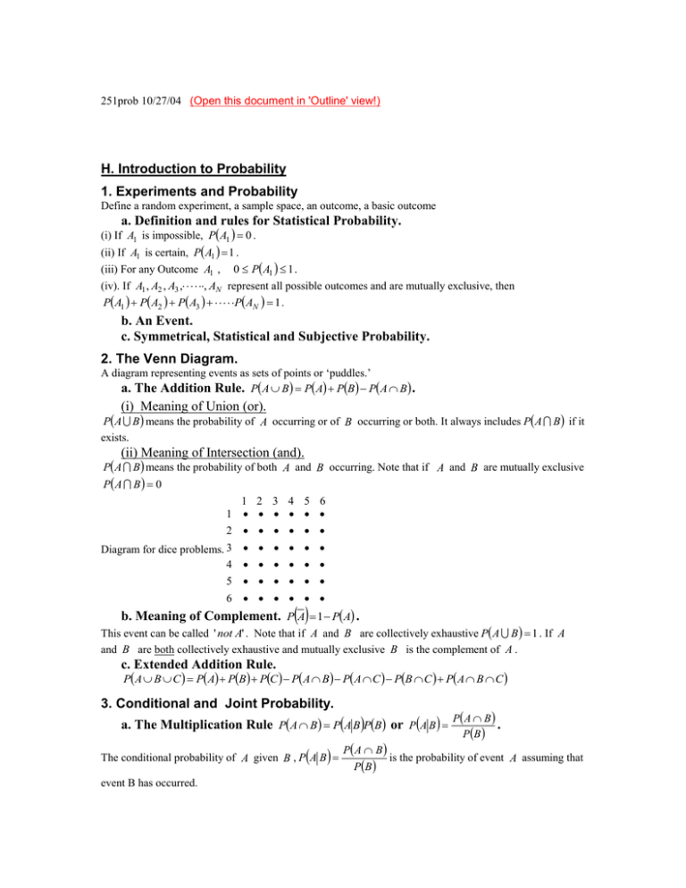
251prob 10/27/04 (Open this document in 'Outline' view!)
H. Introduction to Probability
1. Experiments and Probability
Define a random experiment, a sample space, an outcome, a basic outcome
a. Definition and rules for Statistical Probability.
(i) If A1 is impossible, P A1   0 .
(ii) If A1 is certain, P A1   1 .
0  P A1   1 .
(iv). If A1 , A2 , A3 ,    , AN represent all possible outcomes and are mutually exclusive, then
P A1   P A2   P A3       P AN   1 .
(iii) For any Outcome A1 ,
b. An Event.
c. Symmetrical, Statistical and Subjective Probability.
2. The Venn Diagram.
A diagram representing events as sets of points or ‘puddles.’
a. The Addition Rule. P A  B  P A  PB  P A  B .
(i) Meaning of Union (or).
P A  B  means the probability of A occurring or of B occurring or both. It always includes P A  B  if it
exists.
(ii) Meaning of Intersection (and).
P A  B  means the probability of both A and B occurring. Note that if A and B are mutually exclusive
P A  B   0
1 2 3 4 5 6
1      
2      
Diagram for dice problems. 3      
4      
5      
6      
b. Meaning of Complement. PA  1  PA .
This event can be called ' not A' . Note that if A and B are collectively exhaustive P A  B   1 . If A
and B are both collectively exhaustive and mutually exclusive B is the complement of A .
c. Extended Addition Rule.
P A  B  C   P A  PB   PC   P A  B   P A  C   PB  C   P A  B  C 
3. Conditional and Joint Probability.
a. The Multiplication Rule PA  B  PA BPB or PA B  
The conditional probability of A given B , PA B  
event B has occurred.
P A  B 
P B 
P A  B 
.
P B 
is the probability of event A assuming that
b. A Joint Probability Table.
What is the difference between joint, marginal and conditional probabilities? Remember that we cannot
read a conditional probability directly from a joint probability table but must compute it using the second
version of the Multiplication Rule.
c. Extended Multiplication Rule. PA  B  C   P C A  B P B A PA
d. Bayes' Rule. PB A 

PA B PB 
 
P A
4. Statistical Independence.
a. Definition: PA B  PA
b. Consequence: P A  B   P A PB 
c. Consequence: If A and B are independent so are A and B , A and B etc.
5. Review.
Rule
In General
Multiplication
P A  B 
Addition P A  B 
 
Bayes' Rule P A B
 
Bayes' Rule P B A
 PA B PB 
A and B mutually
exclusive
0
 P APB 
 P A  PB   P A  B 
 P A  PB 
 P A  PB   P APB 
 PB AP A


P B AP A
0
 P A
0
 PB 
P B 
P A B PB 
A and B independent
P  A
I. Permutations and Combinations.
1. Counting Rule for Outcomes.
a. If an experiment has k steps and there are n1 possible outcomes on the first
step, n2 possible outcomes on the second step, etc. up to n k possible outcomes on
the k th step, then the total number of possible outcomes is the product n1n2  nk .
b. Consequence. If there are exactly n outcomes at each step, the total possible
outcomes from k steps is nk .
2. Permutations.
a. The number of ways that one can arrange n objects: n!
b. Prn 
n!
n  r !
Order counts!
3. Combinations.
a. C rn 
n!
n  r !r!
Order doesn't count!
b. Probability of getting a given combination
This is the number of ways of getting the specified combination divided by the total number of possible
combinations. If there are a equally likely ways to get what you want and b equally likely possible
2
outcomes, the probability of getting the outcomes you want is a . Example: If there is only one way to get
b
48
4 jacks from 4 jacks in a poker hand and C1 ways to get another card, a  1C148 The number of ways to
get a poker hand of 5 cards is b  C552 , so the probability of getting a poker hand with 4 jacks is
48
a  C1
.
b
C552
3
J. Random Variables.
1. Definitions.
Discrete and Continuous Random Variables. Finite and infinite populations. Sampling with replacement.
2. Probability Distribution of a Discrete Random Variable.
By this we mean either a table with each possible value of a random variable and the probability of each
value (These probabilities better add to one!) or a formula that will give us these results. We can still speak
of Relative Frequency and define Cumulative Frequency to a point x 0 as the probability up to that point, i.e.
F  x 0   P x  x 0 
3. Expected Value (Expectation) of a Discrete Random
Variable.  x  E x    x  Px  .
Rules for linear functions of a random variable:
a and b are constants. x is a random variable.
a. Eb  b
b. Eax  aEx 
c. Ex  b  Ex  b
d. Eax  b  aEx  b
4. Variance of a Discrete Random Variable.

  
 x2  Varx   E x   2  E x 2   x2
Rules for linear functions of a random Variable:
a. Varb  0
b. Varax  a 2Varx
c. Varx  b  Varx 
d. Varax  b  a 2Varx
Example -- see 251probex1.
5. Summary
a. Rules for Means and Variances of Functions of Random Variables.
251probex4
b. Standardized Random Variables, z 
x

. See 251probex2.
6. Continuous Random Variables.
a. Normal Distribution (Overview).
4
The General formula is f x  
1
 2
1  x 
 

e 2  
2
. Don’t try to memorize or even use this formula. It is
much more important to remember what the normal curve looks like.
5
b. The Continuous Uniform Distribution.
f x  
1
d c
f x   0
cxd
for
otherwise.
xc
for c  x  d , F x   0 for x  c and F x   1 for x  d .
d c
To find probabilities under this distribution, go to 251probex3.
F x  
c. Cumulative Distributions, Means and Variances for Continuous Distributions.
Discrete Distributions
Cumulative Function
F x 0   Px  x 0  
Continuous Distributions
 Px 
F  x 0   P x  x 0  
x  x0
  E x  
Mean
Variance
 xPx 
  E x  

 x2  E x   2


 x    Px 
 Ex   
  x Px  
2


f x dx
x   2 f x dx
 

  x

2
2


x0
xf x dx
 x2  E x   2
2
 E x2   2
2

2

Example: For the Continuous Uniform Distribution, (i) F x 0  
2 



x0  c
d c
d  c 2 .

f x dx   2

(ii)  
cd
and (iii)
2
12
The proofs below are intended only for those who have had calculus!
x0
x0
x c
1
1
1
dx 
dx 
x x xc  0
Proof: (i) F x 0  
0
c d c
c
d c
d c
d c

(ii)   E x  

(iii)  x2  




d
c

d
c
x2
x


1
1 1 2
dx 
x  1 x2  
d c
d  c  2 d 2 c 
1
1 1 3

dx   2 
x
d c 
d  c  3
d

12  dd  cc
2
2

cd 
 13 x 3   


c  2 
cd
2
2
13  d d  cc  14 c 2  2cd  d 2   124 c 2  cd  d 2  123 c 2  2cd  d 2 
3
3
 c
121 c 2  2cd  d 2   d 12
2
6
d. Chebyshef's Inequality Again.
P  k  x    k   1 
1
k2
and don't forget the Empirical Rule
Proof and extensions
7. Skewness and Kurtosis (Short Summary).
Skewness:  3  E x   3 . For a discrete distribution, this means
distribution



 x    Px, and, for a continuous
3
x   3 f x dx
Relative Skewness:  1 
3
3
Kurtosis:  4  E x   4 . For the Normal distribution  4  3 4
Coefficient of Excess:  1 
 4  3 4
4
7