Computer Science Dept.
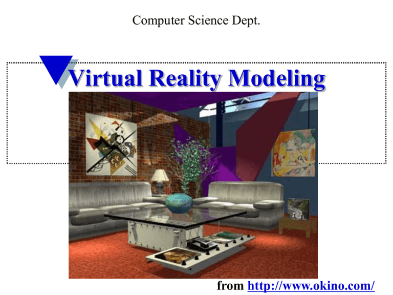
Virtual Reality Modeling
from http://www.okino.com/
Modeling
&
VR Toolkits
System architecture
The VR object modeling cycle:
I/O mapping (drivers);
 Geometric modeling;
 Kinematics modeling;
 Physical modeling;
 Object behavior (intelligent agents);
 Model management.

The VR modeling cycle
The VR geometric modeling:
Object surface shape:
 polygonal meshes (vast majority);
 splines (for curved surfaces);

Object appearance:
Lighting (shading)
 texture mapping

The surface polygonal (triangle) mesh
(X1,Y1,Z1)
(X3,Y3,Z3)
(X5,Y5,Z5)
Non-shared vertex
(X0,Y0,Z0)
(X2,Y2,Z2)
(X4,Y4,Z4)
Shared vertex
Triangle meshes are preferred since they are memory
and computationally efficient (shared vertices)
Object spline-based shape:
 Another way of representing virtual objects;
Functions are of higher degree than linear functions
describing a polygon – use less storage and provide
increased surface smoothness.
 Parametric splines are represented by points x(t), y(t),
z(t), t=[0,1] and a, b, c are constant coefficients.

Object spline-based shape:
Parametric surfaces are extension of parametric splines
with point coordinates given by x(s,t), y(s,t), z(s,t), with
s=[0,1] and t=[0,1].

β-Splines are controlled
indirectly through four
control points (more in
physical modeling section)
Object polygonal shape:
 Can be programmed from scratch using OpenGL or
other toolkit editor; it is tedious and requires skill;
 Can be obtained from CAD files;
Can be created using a 3-D digitizer (stylus), or a 3-D
scanner (tracker, cameras and laser);
 Can be purchased from existing online databases
(Viewpoint database). Files have vertex location and
connectivity information, but are static.

Geometric Modeling
CAD-file based models:
 Done using AutoCAD;
 Each moving part a
separate file;
 Files need to be
converted to formats
compatible with VR
toolkits;
 Advantage – use of
preexisting models in
manufacturing
applications.
Geometric Modeling
Venus de Milo created
using the HyperSpace
3D digitizer, 4200 textured
polygons using NuGraph
toolkit
Case example: Ferrari down-force rear wing
Point cloud from scanner
Polygonal mesh
Virtual wind tunnel
Virtual wind tunnel
http://www.geomagic.com/en/community/casestudies/prodrive-speeds-ferrari-wing-developmentwith-reverse-engineerin/
Polhemus 3-D scanners:
 Eliminate direct contact with object.
uses two cameras, a laser, and magnetic trackers (if movable
objects are scanned)
 Scanning resolution 0.5 mm at 200 mm range;
 Scanning speed is 50 lines/sec;
 Range is 75-680 mm scanner-object range.

Geometric Modeling
Polhemus FastScan 3D scanner (can scan objects up to 3 m long).
DeltaSphere 3000 3D scanner
150º elevation
 Large models need large-volume
Scanners;
 The 3rdTech scanners use time-of-flight
modulated laser beam to determine position.
electrical motor
and CPU
Features:
 Scanning range up to 40 ft;
 Resolution 0.01 in;
360º horizontal
 accuracy 0.3 in;
 scan density of up to 7200 samples/360º;
 complete scene scanning in 10 – 30 minutes (scene has to be
static);
 optional digital color camera (2008x1504 resolution) to add
color to models. Requires a second scan, and reduces elevation to
77º.
www.3rdtech.com
Polhemus scanner
DeltaSphere 3000 3D scanner
Feature
Polhemus scanner
DeltaSphere scanner
Range
0.56 m
14.6 m
Resolution
0.5 mm @ 0.2 m
0.25 mm
Control
manual
automatic
Speed
50 lines/sec
25,000 samples/sec
www.3rdtech.com
DeltaSphere 3000 image
www.3rdtech.com
DeltaSphere 3000 software-compensated image
www.3rdtech.com
Light Detection And Ranging
(LIDAR)
- Optical remote sensing technology that can measure the distance
to, or other properties of a target by illuminating the target
with Light, often using pulses from a laser.
-Geomatics, archaeology, geography, geology, geomorphology, sei
smology, forestry, remote sensing and atmospheric physics.
-Also for 'airborne laser swath mapping' (ALSM), 'laser altimetry'
and LiDAR Contour Mapping.
This LiDAR (laser range finder) may be used
to scan buildings, rock formations, etc., to
produce a 3D model. The LiDAR can aim its
laser beam in a wide range: its head rotates
horizontally, a mirror flips vertically. The laser
beam is used to measure the distance to the
first object on its path.
A FASOR used at the Starfire Optical Range for
LiDAR and laser guide star experiments is
tuned to the sodium D2a line and used to excite
sodium atoms in the upper atmosphere.
How it work?
- A laser generates an optical pulse
- The pulse is reflected off an object and is returned to the instrument
- A high-speed counter measures the time of flight from the start to
the return pulse
- Finally, the time measurement is converted to a distance using the
formula:
R = (T * Э)/2 (1)
Where R = range (m)
T = time of flight(s)
Э = speed of light(m/s)
Three mature technologies are combined in airborne laser mapping:
- laser rangefinder (LiDAR)
- Inertial reference system
(INS) and
- Global positioning system
(GPS).
Hardware
Optech’s Airborne Laser Terrain Mapper
(ALTM)
The ALTM 2050 collects 50,000
measurements per second and has a
maximum altitude of 2000 m.
Maintain balance between scanner
speed and aircraft speed.
Optech's ILRIS-3D tripod-mounted laser scanner.
It has long ranging capabilities (up
to 1000 m)
Obtaining a line of sight that allowed
for economical data collection was
challenging
Two methods were available to fuse
the ground and airborne sensor data:
-Geo referencing the
ground and airborne
data, or
-Aligning both data sets
by identifying common
points.
Fused sensor data:
ILRIS-3D data is grey,
ALTM data is pink
A LiDAR point cloud captured from above can be rotated and
colorized with RGB values from a digital aerial photo to
produce a realistic 3D oblique view
This is a LIDAR map of the Manhattan, New York. This LIDAR map
was used after 9/11 to determine what cranes are necessary to remove
the rubble
http://www.noaanews.noaa.gov/stories/s798.htm
Conversion of scanner data:
Scanners produce a dense “cloud” of vertices (x,y,z).
 Using such packages as Wrap (www.geomagic.com) the point data
are transformed into surface data (including editing and decimation)

Point cloud
from scanner
Polygonal mesh
after decimation
Polygonal
surface
NURBS (non-uniform
rational β-splines) patches
NURBS surface
Geometric Modeling – using online databases
Low res. Model
– 600 polygons
Higher resolution model
> 20,000 polygons.
Geometric Modeling
Object Visual Appearance
 Scene illumination (local or global);
Texture mapping;
 Multi-textures
 Use of textures to do illumination in the rasterizing
stage of the pipeline

Scene illumination
 Local methods (Flat shaded, Gouraud shaded,
Phong shaded) treat objects in isolation. They are
computationally faster than global illumination
methods;
Global illumination treats the influence of one object
on another object’s appearance. It is more demanding
from a computation point of view but produces more
realistic scenes.

Local illumination methods
Ip = Ib – (Ib- Ia) xb-xp
xb-xa
Flat shading model
Gouraud shading model
Phong shading model
Flat shaded
Utah Teapot
Phong shaded
Utah Teapot
Global scene illumination
 The inter-reflections and shadows cast by objects on each
other.
Radiosity illumination
 Results in a more realistic looking scene
Without radiosity
With radiosity
Radiosity illumination
…
but until recently only for fly-through (geometry fixed).
A second process was added so that scene geometry
can be altered
Texture mapping
It is done in the rasterizer phase of the graphics
pipeline, by mapping texture space coordinates to
polygon vertices (or splines), then mapping these to
pixel coordinates;
 Texture increase scene realism;
 Texture provide better 3-D spatial cues (they are
perspective transformed);
 They reduce the number of polygons in the scene –
increased frame rate (example – tree models).

Textured room image for increased realism
from http://www.okino.com/
VR Modeling
The Texturing Functional Sub-Stages
Application
Compute
Object space
Location
Use projector
Function for
Parameter space
Geometry
Corresponder
Function to
Find pixel
Rasterizer
Apply value
Transform
function
Modify
Illumination
equation
How to create textures:
 Models are available on line in texture
“libraries” of cars, people, construction materials, etc.
 Custom textures from scanned photographs or
 Using an interactive paint program to create bitmaps
Texture mapping
[0,1]
Screen space
Object surface
[0,1]
Texture space
256x256 texture
Image Texture:
 It “glues” an image to a polygon.
Size of texture is restricted by graphics accelerators
to 2m  2n or 2m  2m square. The lower limit for
OpenGL is 64  64 texels.
 If the size of the polygon is much larger than the size
of the texture then the hardware has to perform
Magnification;
 If there are much fewer pixels than texels – minification;
 Both techniques use bilinear interpolation to assign colors
to pixels.

VR Geometric Modeling
Tree,
higher resolution model
45,992 polygons.
Tree represented as a texture
1 polygon, 1246x1280 pixels
(www.imagecels.com).
Multi-texturing:
 Several texels can be overlaid on one pixel;
 A texture
blending cascade is made up of a series of texture stages
Interpolated
vertex values
Polygon/
Stage 0
Stage 1
Stage 2
Texture
value 0
Texture
Texture
value 1
value 2
(from “Real Time Rendering”)
Image buffer
Allow more complex textures
Normal
texture
Background
texture
Reflectivity
texture
Transparency
texture
Bump
maps
Multi-texturing for bump mapping:
 Lighting effects caused by irregularities on object
surface are simulated through “bump mapping”;
 This encodes surface irregularities as textures;
 No change in model geometry. No added
computations at the geometry stage;
 Done as part of the per-pixel shading operations
of the Nvidia Shading Rasterizer
Bump mapping per-pixel shading
VC 5.1
Normal
texture
Multitexture
Bump
texture
Multi-texturing for lighting:
 Several texels can be overlaid on one pixel;
One application in more realistic lighting;
 Polygonal lighting is real-time but requires lots of
polygons (triangles) for realistic appearance

Vertex lighting of low polygon
count surface – lights are diffuse –
tessellated.
Vertex lighting of high polygon
count surface – lights have realistic
appearance. High computation load
(from NVIDIA technical brief)
Multi-texturing (texture blending):
 Realistic-looking lighting can be done with
2-D textures called “light maps”;
 Not applicable to real-time (need to be recomputed
when object moves)
Standard lighting map
2-D texture
Light map texture overlaid
on top of wall texture. Realistic
and low polygon count. Not real-time!
(from NVIDIA technical brief)
NVIDIA Shading Rasterizer:
 NVIDIA proposed to combine the dynamics of Polygon-based


shading with the realism of light maps;
Vertex info used in shading: position, texture, normal;
Let’s assign same info to pixels and do shading at pixel level!
Lighting in Geometry Stage
Lighting by interpolation
of vertex information
Lighting with Shading Rasterizer
Realistic and real-time!
(from NVIDIA technical brief)
NVIDIA Shading Rasterizer (NSR):
Texels contain information about position and color;
 We still need information about normals – special type
of texture called “normal map”
 texel information + normal maps are used to calculate light
intensity and direction on a per-pixel basis;
 Texture blending operations allow real-time diffuse,
spot and point light effects for each pixel;
 Much faster. NVIDIA Quadro2 can render in real time
frames that took hours of off-line rendering for Pixar’s
A Bug’s Life.

(from NVIDIA technical brief)
VR Kinematics Modeling:
Homogeneous transformation matrices;
 Object position;
 Transformation invariants;
 Object hierarchies;
 Viewing the 3-D world.

VR Modeling
The Graphics Rendering Pipeline (revisited)
Application
Geometry
Rasterizer
The Geometry Functional Sub-Stages
Model & View
Transformation
Lighting
Projection
Clipping
Screen
Mapping
VR Modeling
The Rendering Pipeline
Application
Geometry
Rasterizer
The Geometry Functional Sub-Stages
Model & View
Transformation
Lighting
Projection
Clipping
Screen
Mapping
Model and Viewing Transformations:
 Model transforms link object coordinates to world
coordinates. By changing the model transform, the same
object can appear several times in the scene.
We call these instances.
[
1
0
0
0
0
1
0
0
Virtual ball
0 p1x (t)
0 p1y (t)
1 p1z (t)
0 1
World system of coordinate
]
Instance 2 of Virtual ball
Instance 5
[
1
0
0
0
0
1
0
0
0 p5x (t)
0 p5y (t)
1 p5z (t)
0 1
]
Camera system of coordinates
y T camera  fingertip 2 (t)
z
x
T camera  fingertip 1 (t)
The View Transform matrix captures
the position and orientation of the
virtual camera in the virtual world;
 It maps world coordinates to camera
space (also called “eye space”);
 The camera is located at the origin of
the camera coordinate system, looking in the negative Z axis,
with Y pointing upwards, and X to the right.
y
Camera “fly-by”
z
x
T camera  tree (t)
User interactively changes the
viewing transform by changing
the position and aim of the virtual
camera = “fly-by.” Example –
NVIDIA Grove demo. This demo
Also shows instances
VR Modeling
The Rendering Pipeline
Application
Geometry
Rasterizer
The Geometry Functional Sub-Stages
Model & View
Transformation
Lighting
Projection
Clipping
Screen
Mapping
Projection Transformations:
 Models what portion (volume) of the virtual world the
camera actually sees. There are two kinds of projections,
parallel projection and perspective projection. VR uses
perspective.
projection plane
projection reference point
Parallel projection
Perspective projection
Perspective Projection Transformation:
If the projection reference point is at the origin of the system of
coordinates, and the projection plane is at –d,
Then the (non invertible) perspective projection transformation
matrix is:

T projection=
1
0
0
0
[
0 0
1 0
0 1
0 -1/d
0
0
0
0
]
projection plane
Y
projection reference point
-d
Z
X
Second Perspective Projection Transformation:
The portion of the virtual world seen by the camera at a given
time is limited by front and back “clipping planes”.
These are at z=n and z= f. Only what is within the viewing cone
(also called fulcrum) is sent down the rendering pipe.

clipping plane
(l,t,f)
Y
projection reference point
(r,b,n)
Z
X
Canonical Mapping:
The second projection transform maps the viewing volume to a
unit cube with extreme points at (-1,-1,-1) and (1,1,1). This is called
the canonical view volume.

[
T’ projection=
2n/(r-l) 0
-(r+l)/(r-l)
0
0
2n/(t-b) -(t+b)/(t-b)
0
0
0
(f+n)/(f-n) -2fn/(f-n)
0
0
1
0
]
(l,t,f)
Y
Y
X
Z
X
(r,b,n)
Z
VR Modeling
The Rendering Pipeline
Application
Geometry
Rasterizer
The Geometry Functional Sub-Stages
Model & View
Transformation
Lighting
Projection
Clipping
Screen
Mapping
Clipping Transformation:
Since the fulcrum maps to the unit cube, only objects inside it
will be rendered. Some objects are partly inside the unit cube (ex.
the line and the rectangle). Then they need to be “clipped”. The
vertex V1 is replaced by new one at the intersection between the
line and the viewing cone, etc.

V1 Scene clipping
Unit cube
V1
X
X
V2
V2
V3
V3
Z
Z
VR Modeling
The Rendering Pipeline
Application
Geometry
Rasterizer
The Geometry Functional Sub-Stages
Model & View
Transformation
Lighting
Projection
Clipping
Screen
Mapping
Screen Mapping (Viewport Transformation):
The scene is rendered into a window with corners (x1,y1), (x2,y2)
 Screen mapping is a translation followed by a scaling that affects
the x and y coordinates of the primitives (objects), but not their z
coordinates. Screen coordinates plus z [-1,1] are passed to the
rasterizer stage of the pipeline.

Screen mapping
V1
(x2,y2)
X
V2
V3
Z
(x1,y1)
KINEMATICS MODELING:
Homogeneous transformation matrices;
 Object position;
 Transformation invariants;
Object hierarchies;
 Viewing the 3-D world.

Homogeneous Transformations:
 Homogeneous system of coordinates is a
right-hand Cartesian system of coordinates with
orthonormal unit vector triads;
 Such (i, j, k) triads have the property that their
norms |i|= |j| = |k| = 1 and their dot product is
i • j = i • k = j • k = 0;
 Homogeneous transformation matrices relate two
such systems through a 4  4 matrix.
Homogeneous Transformations:
 Have the general format:
T A B =
[
R3x3
0
0
0
]
P3x1
1
where R3x3 is the rotation submatrix expressing the orientation
of the system of coordinates B vs. system of coordinates A;
P3x1 is the position vector of the origin of system B
vs. the origin of system of coordinates A.
Homogeneous Transformations:
Have many advantages:
 treat object translation and rotation mathematically
in the same way;
 are easily invertible;

T B  A = ( T A  B ) -1 =
[
RT
0
0
-RT  P
0
1
]
Object Position/Orientation (static):
 given by homogeneous transformation matrix
that relates the object system of coordinates to
world system of coordinates.
T W1 =
[
]
iw1 jw1 kw1 P1
0
0
0
1
where iw1 , jw1 , kw1 are
3  1 vectors projecting the object unit
vectors into world system of coordinates
Object Position/Orientation (moving):
 If the virtual object moves, then the
transformation matrix becomes a function of time
T W  1 (t) =
[
]
iw1 (t) jw1(t) kw1(t) P1 (t)
0
0
0
1
The position of an object vertex Vi in world
coordinates versus its position in object coordinates
Vi(W) (t) = T W  1 (t) Vi (object)
If the aligned virtual object translates, all vertices
translate
Vi(W) (t) =
[
1
0
0
0
0
1
0
0
0 p1x (t)
0 p1y (t)
1 p1z (t)
0
1
]
Vi (object)
If the virtual object translates back to its initial position,
all its vertices translate by an equal but negative amount.
Vi(W) (t) =
[
1
0
0
0
0
1
0
0
0 -p1x (t)
0 -p1y (t)
1 -p1z (t)
0
1
]
Vi (object)
If the virtual object needs to be scaled, it is translated
to origin, scaled, then translated to back
Vi(W) (t) = T W  2
[
si
0
0
0
0
sj
0
0
0
0
sk
0
0
0
0
1
]
T W  1Vi (object)
Tracking a virtual hand:
Object system of coordinates
Source system of coordinates
T sourcereceiver
T worldsource
T worldobject
Receiver system of coordinates
World system of coordinates
Transformations concatenation:
 Transformation matrices can be compounded to
obtain the resulting motion. Example – simulating
a virtual hand.
T W  hand (t) = T W  source T source  receiver (t)
 If the object is grasped, then its position does not
change vs. the hand. Thus the movement of the
grasped object in word coordinates is:
T W  object (t) = T W  source T source  receiver (t) T receiver object
VR Kinematics Modeling
Object Hierarchies:
 Allows models to be partitioned into a hierarchy,
and become dynamic;
 Segments are either parent (higher level object)
or child (lower level objects).
 The motion of a parent is replicated by its
children but not the other way around.
 Example – the virtual human and the virtual
hand;
 At the top of the hierarchy is the “world global
transformation” that determines the view to the scene.
VR Kinematics Modeling
a)
b)
Model hierarchy: a) static model (Viewpoint Datalabs);
b) segmented model.
Object hierarchy for a Virtual Hand:
 Transformation matrices can be compounded to obtain the
motion of the fingertip versus the world coordinates.
T global  fingertip (t) = T global W(t) T W source T source palm (t) 
T palm 1 (t)T 1 2 (t) T 2 3 (t) T 3 fingertip
T W palm (t) is given by the glove tracker
T palm 1 (t), T 1 2 (t), T 2 3 (t) are given by the sensors on
the glove
T 3 fingertip
Camera system of coordinates
y T global  fingertip (t)
T 2 3 (t)
T 1 2 (t),
z
x
T palm 1 (t)
T global W(t)
T source palm (t)
T W source
Receiver system
of coordinates
Source system of coordinates
World system of coordinates
T global  fingertip (t) = T global W(t) T W source T source palm (t) 
T palm 1 (t)T 1 2 (t) T 2 3 (t) T 3 fingertip
Camera system of coordinates
y
z
x
T global  car(t)
Vicar
T global W(t)
World system of coordinates
T global  vertex(i) (t)= T global W (t)T W car (t) Vi
Vicar
The VR physical modeling:
from (Burdea 1996)
The Haptics Rendering Pipeline (revisited)
Traversal
Collision
Detection
Force
Force
Calculation
Application
Scene
Traversal
Force
Smoothing
Tactile
Force
Mapping
Geometry
View
Transform
Lighting
Display
Haptic
Texturing
Rasterizer Display
Projection
Texturing
adapted from (Popescu, 2001)
The Haptics Rendering Pipeline
Traversal
Collision
Detection
Force
Force
Calculation
Force
Smoothing
Tactile
Force
Mapping
Haptic
Texturing
Display
Collision detection:
Uses bounding box collision detection for fast response;
 Two types of bounding boxes, with fixed size or variable
size (depending on enclosed object orientation).
 Fixed size is computationally faster, but less precise

Variable size Bounding Box
Fixed size Bounding Box
Collision Detection
Undetected collision
Ball at time t
Longest distance
Ball at time t + 1/fps
If longest distance d < v • 1/fps
then collision is undetected (v is the ball
velocity along its trajectory)
Two-stage collision detection:
For more precise detection, we use a two-stage collision
detection: an approximate (bounding box ) stage, followed
by a slower exact collision detection stage.

Bounding Box Pruning
multi-body pairs
Simulation
no
Collision response
yes
Pair-wise exact
Collision Detection
yes
Exact collision detection
Surface cutting:
 An extreme case of surface “deformation” is surface cutting. This
happens when the contact force exceed a given threshold;
 When cutting, one vertex gets a co-located twin. Subsequently
the twin vertices separate based on spring/damper laws and the cut
enlarges.
Mesh before cut
V1
Cutting instrument
V2
Mesh after cut
V1
V2
Collision response – surface deformation
The Haptics Rendering Pipeline
Traversal
Collision
Detection
Force
Force
Calculation
Force
Smoothing
Tactile
Force
Mapping
Haptic
Texturing
Display
Haptic interface
Haptic Interface Point
I -Haptic Interface Point
Haptic Interface Point
Penetration distance
Object polygon
Force output for homogeneous elastic objects
{
F=
K • d,
for 0  d  d max
F max
for d max  d
where F max is that haptic interface maximum output force
saturation
F max
d max 1
d max 2
Penetration distance d
Force Calculation –
Elastic objects with harder interior
{
F=
K 1 • d,
for 0  d  d discontinuity
K 1 • d discontinuity + K 2 • (d –d discontinuity), for d discontinuity  d
F max
for d max  d
where d discontinuity is object stiffness change point
F max
F
d discontinuity
d max
Penetration distance d
Force Calculation –
Virtual pushbutton
F = K 1 • d (1-um) +
Fr • u m +
K 2 • (d – n) un
where um and un are unit step
functions at m and n
F
Virtual wall
Fr
m
n
Penetration distance d
Force Calculation –
Plastic deformation
m
F initial = K • d for 0  d  m
F
= 0 during relaxation,
m
n
F subsequent = K 1 • d • um for 0  d  n
F
= 0 during relaxation,
where um is unit step function at m
Moving into the wall
Virtual wall
V0
F
Force Calculation –
Virtual wall
time
Virtual wall
Moving away from the wall
V0
Generate energy due to sampling timeTo avoid system instabilities we add a
damping term
F
{
F=
K wall •  x + B v,
for v  0
K wall •  x,
for v  0
where B is a directional damper
time
The Haptics Rendering Pipeline
Traversal
Collision
Detection
Force
Force
Calculation
Force
Smoothing
Tactile
Force
Mapping
Haptic
Texturing
Display
Force shading:
Non-shaded contact
forces
F smoothed =
Real cylinder contact
forces
{
Contact forces after
shading
K object • d • N , for 0  d  d max
F max • N,
for d max < d
where N is the direction of the contact force based on
vertex normal interpolation
The haptic mesh:
 A single HIP (haptic interface point) is not sufficient to
capture the geometry of fingertip-object contact;
 The curvature of the fingertip, and the object
deformation need to be realistically modeled.
Screen sequence for squeezing an elastic virtual ball
Haptic mesh
Mesh point i
Penetration distance
for mesh point i
Haptic mesh force calculation
Penetration distance
for mesh point i
Haptic Interface Point i
For each haptic interface point of the mesh:
F haptic-mesh i = K object • d mesh i • N surface
where d mesh i are the interpenetrating distances at the
mesh points, N surface is the weighted surface normal
of the contact polygon
The Haptics Rendering Pipeline
Traversal
Collision
Detection
Force
Force
Calculation
Force
Smoothing
Tactile
Force
Mapping
Haptic
Texturing
Display
Force mapping
VC 5.2
Force displayed by the Rutgers Master II interface:
F displayed = ( Fhaptic-mesh )/cos
where  it the angle between the mesh force resultant and the piston
The Haptics Rendering Pipeline
Traversal
Collision
Detection
Force
Force
Calculation
Force
Smoothing
Tactile
Force
Mapping
Haptic
Texturing
Display
Surface haptic texture produced by the PHANToM
interface
Haptic interface
Haptic Interface Point
Y
F texture = A sin(m x) • sin(n y),
X
Z
Object polygon
where A, m, n are constants:
 A gives magnitude of vibrations;
 m and n modulate the frequency of
vibrations in the x and y directions
BEHAVIOR MODELING
 The simulation level of autonomy (LOA) is a function of its
components
 Thalmann et al. (2000) distinguish three levels of autonomy. The
simulation components can be either “guided” (lowest),
“programmed” (intermediate) and “autonomous (high)
Simulation LOA = f(LOA(Objects),LOA(Agents),LOA(Groups))
Simulation
Autonomous
Autonomous
Autonomous
LOA
Programmed
Programmed
Programmed
Guided
Guided
Guided
Interactive object
Intelligent agent
Group of agents
adapted from (Thalmann et al., 2000)
Interactive objects:
 Have behavior independent of user’s input (ex. clock);
This is needed in large virtual environments, where it is
impossible for the user to provide all required inputs.

System clock
Automatic door –
reflex behavior
Interactive objects:
 The fireflies in NVIDIA’s Grove have behavior
independent of user’s input. User controls the virtual
camera;
Agent behavior:
 A behavior model composed of perception, emotions,
behavior, and actions;
 Perception (through virtual sensors) makes the agent
aware of his surroundings.
Perception
Emotions
Behavior
Actions
Virtual world
Avatar
 Written
in 1994
– Development Inspired By Lord of the
Rings
 Goal: animation technology that allows for
close-up shots surpassing uncanny valley
The Uncanny Valley
Avatar Technology



Full Body Motion Capture
– Used for both actors and other in world objects as stand
ins
Facial Motion Capture
– Imparts human emotion to facial animation
Director’s Camera
– Low resolution view of virtual world
Facial Capture
L.A. Noir
 1940’s
Detective Game
– Witness interrogation
 Incorporates Facial motion capture
technology
– Does not require facial markers
References







http://www.gametrailers.com/video/developer-diary-l-anoire/708504
http://www.youtube.com/watch?v=O6OKMhSlSIY&feature=relate
d
http://www.moviemobsters.com/2009/07/18/monster-madnesscreature-4/
http://en.wikipedia.org/wiki/Avatar_%282009_film%29
http://en.wikipedia.org/wiki/L.A._Noire
http://www.twin-pixels.com/the-making-of-avatar-some-juicydetails/
http://www.twin-pixels.com/software-used-making-of-avatar/
Reflex behavior:
 A direct link between perception and actions (following

behavior rules (“cells”);
Does not involve emotions.
Perception
Emotions
Behavior
Actions
Object behavior
Autonomous virtual human
User-controlled hand avatar
Another example of reflex behavior – “Dexter” at MIT
[Johnson, 1991]: Hand shake, followed by head turn
Agent behavior avatars
User-controlled body avatar
Autonomous virtual human
If user maps to a full-body avatar, then virtual human agents react through
body expression recognition: example dance. Swiss Institute of Technology, 1999
(credit Daniel Thalmann)
Emotional behavior:
 A subjective strong feeling (anger, fear) following perception;
Two different agents can have different emotions to the same
perception, thus they can have different actions.

Emotions 1
Perception
Perception
Emotions 2
Behavior
Behavior
Actions 1
Actions 2
Virtual world
Crowds behavior
 Crowd behavior emphasizes group (rather than individual)
actions;
 Crowds can have guided LOA, when their behavior is defined
explicitly by the user;
 Or they can have Autonomous LOA with behaviors specified
by rules and other complex methods (including memory).
Political demonstration
Guided crowd
User needs to specify
Intermediate path points
VC 5.3
Autonomous crowd
Group perceives info on
its environment and
decides a path to follow
to reach the goal
(Thalmann et al., 2000)
MODEL MANAGEMENT
 It is necessary to maintain interactivity and
constant frame rates when rendering complex
models. Several techniques exist:
 Level of detail segmentation;
 Cell segmentation;
 Off-line computations;
 Lighting and bump mapping at rendering
stage;
 Portals.
Level of detail segmentation:
 Level of detail (LOD) relates to the number of polygons
on the object’s surface. Even if the object has high
complexity, its detail may not be visible if the object is
too far from the virtual camera (observer).
Tree with 27,000 polygons
(details are not perceived)
Tree with 27,000 polygons
Static level of detail management:
 Then we should use a simplified version of the object
(fewer polygons), when it is far from the camera.
 There are several approaches:
 Discrete geometry LOD;
 Alpha LOD;
 Geometric morphing (“geo-morph”) LOD.
Discrete Geometry LOD:
 Uses several discrete models of the same virtual object;

Models are switched based on their distance from the
camera (r  r0; r0  r  r1; r1  r  r2; r2  r)
r1
r2
r0
LOD 0
LOD 1
LOD 2
Alpha Blending LOD:
 Discrete LOD have problems on the r0 = r, r1 = r, r2 = r circles,
leading to “popping”. Objects appear and disappear suddenly. One
solution is distance hystheresis. Another solution is model blending –
two models are rendered near the circles;
 Another solution to popping is alpha blending by changing the
transparency of the object. Fully transparent objects are not rendered.
Hystheresis zone
r1
r2
r0
LOD 0
Opaque
LOD 1
Less opaque
LOD 2
Fully transparent
Geometric Morphing LOD:
 Unlike geometric LOD, which uses several models of the same
object, geometric morphing uses only one complex model.
 Various LOD are obtained from the base model through mesh
simplification
 A triangulated polygon mesh: n vertices has 2n faces and 3n edges
Mesh before simplification
V1
Mesh after simplification
V2
V1
Collapsing edges
Single-Object adaptive level of detail LOD:
 Used where there is a single highly complex object that the user
wants to inspect (such as in interactive scientific visualization.
 Static LOD will not work since detail is lost where neededexample the sphere on the right loses shadow sharpness after LOD
simplification.
Sphere with 8192 triangles
– Uniform high density
Sphere with 512 triangles –
Static LOD simplification
(from Xia et al, 1997)
Single-object Adaptive Level of Detail
Sometimes edge collapse leads to problems, so vertices need
to be split again to regain detail where needed. Xia et al. (1997)
developed an adaptive algorithm that determines the level of detail
based on distance to viewer as well as normal direction (lighting).
Refined Mesh
Simplified Mesh
Edge collapse
V1
V2
V1
Vertex Split
V1 is the “parent” vertex
(adapted from Xia et al, 1997)
Single-object Adaptive Level of Detail
Sphere with 8192 triangles
– Uniform high density,
0.115 sec to render
Sphere with 537 triangles
– adaptive LOD, 0.024 sec
to render (SGI RE2, single
R10000 workstation)
(from Xia et al, 1997)
Single-object Adaptive Level of Detail
Bunny with 69,451
triangles – Uniform high
density, 0.420 sec to render
Bunny with 3615 triangles
– adaptive LOD, 0.110 sec
to render (SGI RE2, single
R10000 workstation)
(from Xia et al, 1997)
Static LOD:
 Geometric LOD, alpha blending and morphing have problems
maintaining a constant frame rate. This happens when new complex
objects appear suddenly in the scene (fulcrum).
frame i+1
frame i
fulcrum
Camera “fly-by”
LOD 1
LOD 1
LOD 2
LOD 2
Architectural “walk-through”
(UC Berkeley Soda Hall)
Camera path through auditorium
Start
A
C
End
No LOD menegament, 72,570 polygons
B
Time 1.0 sec
Time 0.2 sec
A
A
C
B
B
0
Frames
C
250
0
No LOD management
Frames
250
Static LOD management
from (Funkhauser and Sequin, 1993)
Adaptive LOD Management-continued:
 An algorithm that selects LOD of visible objects based on a
specified frame rate;
 The algorithm (Funkhauser and Sequin, 1993) is based on a
benefits to cost analysis, where cost is the time needed to render
Object O at level of detail L, and rendering mode R.

The cost for the whole scene is
 Cost (O,L,R)  Target frame time

where the cost for a single object is
Cost (O,L,R) = max (c1Polygons(O,L) + c2 Vertices(O,L), c3 Pixels(O,L))
c1, c2, c3 are experimental constants, depending on R and type of computer
Adaptive LOD Management:
 Similarly the benefit for a scene is a sum of visible
objects benefits;
 Benefit(O,L,R)
 where the benefit of a given object is
Benefit(O,L,R) = size(O) * Accuracy(O,L,R) * Importance(O) * Focus(O) *
Motion(O) * Hysteresis(O,L,R)

The algorithm tries to maximize each object’s “value”
Value= Benefit(O,L,R)/Cost(O,L,R)
Objects
with higher value (larger size) are rendered first
A
C
No detail elision, 72,570 polygons
Optimization algorithm, 5,300 poly.
0.1 sec target frame time (10 fps)
from (Funkhauser and Sequin, 1993)
Cell segmentation:
It is another method of model management,
used in architectural walk-through;
 To maintain the “virtual building” illusion it
is necessary to have at least 6 fps (Airey et al., 1990)
 Necessary to maintain interactivity and
constant frame rates when rendering complex
models.

The Visibility Problem
Given the current view
point and the viewing
direction.
We would like to render
the visible portion of the
model and as little as
possible of the rest of
the model.
Model management
Only the current “universe” needs to be rendered
Cells and Portals
Cells:
Regions whose boundary is
formed by a sequence of walls
and portals.
For example: rooms.
Portals:
Transparent doorways
connecting two cells, filling the
missing portions of the cells
boundary.
For example: doors.
Cell segmentation – increased frame rate
 Buildings are large models that can be partitioned in “cells”
automatically and off-line to speed up simulations at run time;
 Cells approximate rooms;
 Partitioning algorithms use a “priority” factor that favors
occlusions (partitioning along walls)
Binary Space Partition
(BSP) tree
Automatic floor plan partition (Airey et al., 1990)
BSP Trees Algorithm
•Choose a splitting plane.
Use the plane to split the
space into two.
•Repeat recursively for both
subspaces.
•The end result is a binary
tree whose leafs are convex
spaces, which are the cells.
Rendering the cells
Cells and Portals work under the assumption that the
model is hidden and that the visible parts should be
discovered.
The current cell
Visible cells
Hidden cells
Usually, visibility algorithms
assume the model is visible and
that the hidden parts should be
removed.
Rendering the cells
Run a Depth First Search
from the current cell.
Test the portals. If a portal is
visible, clip it and move to
the adjacent cell.
Render the cells that were
visited during the traversal.
Breaking the Wall Algorithm



The algorithm works in 2D.
The edges given to the
algorithm are extracted from
the 3D model. They are single
sided and oriented.
Similarly, the created cells can
be given height and associated
with 3D model.
Input
Model
Extracted
Edges
Breaking the Wall Algorithm




Uses a adjacency graphCells are nodes and portals are
branches
The set of Cells that are visible from
the current view point is found
through a recursive depth-first
traversal of the adjacency graph.
When applying the algorithm only
the geometry from the partially
visible cells is sent to the graphics
pipeline
Breaking the Wall Algorithm
Initial partition:
Create cells with short
portals relative to wall
size.
Final partition:
Refine the partition,
creating smaller cells that
have short portals
relative to cell size.
Creating the initial Partition
Traverse the walls (ccw),
creating portals wherever
necessary.
o
Whenever the path
intersects itself, a cell is
created. Remove the cell
from the path and continue.
o
Repeat the process until
all the walls have been
assigned to cells.
o
Going outdoors
Render with
frustum culling
Splitting height
Render
with cells
and portals
Going outdoors
Create a ground
partition.
 Create a roof-top
partition.
 Merge the partitions
and extend the portals.

Evaluating the Partitions Quality
BSP Partition
BW Partition
We applied the second pass
of the BW algorithm (the
refinement pass) to the cells
of the BSP tree.
A “Merged BSP” partition
is created, to which we
compared the BW
algorithm.
“Merged BSP” Partition
Evaluating the Partitions Quality
Model
Soda
London
Sava
Method
Avg.
#visible
cells
Avg. #
portals
tested
Avg. area
rendered
BW
8
25
106.247
“Merged BSP”
12
85
116.739
BW
25
83
72.551
“Merged BSP”
28
609
107.986
BW
18
62
956.454
“Merged BSP”
23
372
1959.15
Cell segmentation
Frame time (s)
 Building model resides in a fully associative cache;
 But cell segmentation alone will not work if the model is so large
that it exceeds available RAM;
 In this case large delays will occur when there is a page fault and
data has to be retrieved from hard disk;
Page faults
From (Funkhauser, 1993)
Frames
Combined Cell, LOD and database
methods
 It is possible to add database management techniques to prevent
page faults and improve fps uniformity during walk-through;
 It is possible to estimate how far the virtual camera will rotate and
translate over the next N frames and pre-fetch from the hard disk the
appropriate objects.
Visibility
Detail
Determ.
Ellision
Lookahead
Determ.
Cache
Management
Render
Monitor
User
Interface
I/O
Oper
Database
Database management
Floor plan partition (Funkhouser, 1993)
Database management
LOD 0
LOD 1
LOD 2
LOD 3
LOD 1
LOD 0 – highest level of detail (loaded first)
….
LOD 3 - lowest level of detail (loaded last)
LOD 2
LOD 3
LOD 2
LOD 3
Frame time (s)
LOD 3
Frames
Floor plan visibility and highest LOD (Funkhouser, 1990)