STA 6207 – Exam 2 – Fall 2012
PRINT Name _____________________
Conduct all tests at  = 0.05 significance level.
All Questions are based on the following 2 regression models, where SIMPLE REGRESSION refers to
the case where p=1, and X is of full column rank (no linear dependencies among predictor variables).
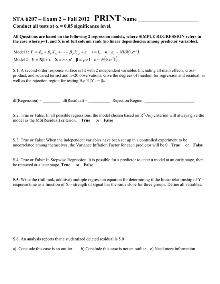
Model 1 : Yi   0  1 X i1     p X ip   i

i  1,..., n  i ~ NID 0,  2

Model 2 : Y  Xβ  ε X  n  p' β  p'1 ε ~ N 0,  2 I


S.1. A second-order response surface is fit with 2 independent variables (including all main effects, crossproduct, and squared terms) and n=20 observations. Give the degrees of freedom for regression and residual, as
well as the rejection region for testing H0: E{Y} = 0
df(Regression) = ________ df(Residual) = __________ Rejection Region: _______________________
S.2. True or False: In all possible regressions, the model chosen based on R2-Adj criterion will always give the
model as the MS(Residual) criterion. True or False
S.3. True or False: When the independent variables have been set up in a controlled experiment to be
uncorrelated among themselves, the Variance Inflation Factor for each predictor will be 0. True or False
S.4. True or False: In Stepwise Regression, it is possible for a predictor to enter a model at an early stage, then
be removed at a later stage. True or False
S.5. Write the (full rank, additive) multiple regression equation for determining if the linear relationship of Y =
response time as a function of X = strength of signal has the same slope for three groups. Define all variables.
S.6. An analysis reports that a studentized deleted residual is 5.0
a) Conclude this case is an outlier
b) Conclude this case is not an outlier
c) Need more information
Q.1. A research firm is interested in the effects of 3 types of advertising (Newspaper, and Internet) on a firm’s
sales. They hold all other variables constant over the study period (such as price and store promotion). The
sample is based on n=6 sales periods. They fit the following 2 regressions.
Model 1: E Y   0   N N   I I
Model 2 : E Y   0   A A
A N I
Model 1
X0
1
1
1
1
1
1
Model 2
X0
1
1
1
1
1
1
X1
1
2
3
1
2
3
X1+X2
2
3
4
4
5
6
X2
1
1
1
3
3
3
Y
5
6
9
7
9
12
Y
5
6
9
7
9
12
X'X
6
12
12
12
28
24
12
24
30
INV(X'X)
1.833333
-0.5
-0.33333
-0.5
0.25
0
-0.33333
0
0.166667
Y'Y
416
Y'(1/n)JY
384
X'X
6
24
24
106
X'Y
48
209
INV(X'X)
1.766667
-0.4
-0.4
0.1
beta-hat
1.2
1.7
^
p.1.a. Show that Y'PY = β'X'Y
p1.b. Compute SS(Total Corrected), SS(Reg1) and SS(Res1)
p.1.c. Test H0: N = I = 0
at  = 0.05 significance level.
Test Statistic ____________________________ Rejection Region ___________________________
p1.d. Compute SS(Reg2) and SS(Res2)
p.1.e. Test H0: N = I at  = 0.05 significance level.
Test Statistic ___________________________ Rejection Region __________________________
Q.2. A simple regression model is fit, relating a dependent variable Y, to an independent variable X. You are
given the following data and summary statistics.
X
0
0
0
10
10
10
20
20
20
Y
15
13
17
25
27
23
34
32
39
Y-hat_j
Y-bar_j
sum(X)
90
sum(Y)
225
SS_XX
600
SS_YY
642
SS_XY
600
p.2.a. Give the fitted equation, based on the simple linear regression model:
^
^
^
 1  _______________________  0  _______________________ Y  ____________________
p.2.b. Fill in the 3rd and 4th columns of the table above.
p.2.c. Compute the Pure Error Sum of Squares and degrees of freedom:
SSPE = _______________________________________________ dfPE = ________________________
p.2.d. Compute the Lack-of-Fit Sum of Squares and degrees of freedom:
SSLF = _______________________________________________ dfLF = ________________________
p.2.e. Test H0: Model is Linear vs HA: Model is not Linear at  = 0.05 significance level.
Test Statistic _____________________________ Rejection Region __________________________
Q.3. A regression model is fit, relating the number of breeding pairs of penguins to the year, over a period of
years. The researchers use Y= log10(# breeding pairs) and X = (Year – mean(Year)) . They fit 3 Models:
Model 1: E Y   0
Model 2: E Y   0 +1 X
Model1
beta-hat
4.4197
Model2
beta-hat
4.4197
0.0199
Model3
beta-hat
4.5390
0.0095
-0.0012
X'Y
48.6162
X'Y
48.6162
21.0521
X'Y
48.6162
21.0521
4300.8246
Model 3: E Y   0 +1 X  2 X 2
p.3.a. Compute R(0), R(0, ), R(0, 2), R(0), and R(0, ) (use 4 decimal places)
R(0) = ____________________ R(0, ) = __________________ R(0, 2)_________________
R(0) = ______________________________ R(0, ) = _____________________________
p.3.b. Compute the fitted values and residuals for the following years, for each model:
Year
1981
1989
1998
X
-9.09
-1.09
7.91
Y
4.17
4.62
4.41
Fit1
Residual1
Fit2
Residual2
Fit3
Residual3
Q.4. A linear regression model is fit, relating apartment rental prices (Y, in $100) to square footage for for 5
apartments in each of 4 luxury neighborhoods (all apartments were built in the same decade). We consider the
following 3 models, where X1 is the square footage (100s of ft2); X2 =1 if neighborhood A, 0 otherwise; X3=1 if
neighborhood B, 0 otherwise; and X4=1 if neighborhood C, 0 otherwise.
Model 1: E Y    0  1 X 1
Model 2: E Y    0  1 X 1   2 X 2  3 X 3   4 X 4
Model 3: E Y    0  1 X 1   2 X 2  3 X 3   4 X 4  5 X 1 X 2   6 X 1 X 3   7 X 1 X 4
The ANOVA Tables from each model are given below.
ANOVA
Model1
df
Regression
1
Residual
18
Total
19
SS
201.2
90.3
291.4
Model2
df
4
15
19
SS
228.7
62.7
291.4
Model3
df
7
12
19
SS
249.6
41.8
291.4
p.4.a. Test whether the “square footage effect” is the same for each neighborhood by completing the following
parts (homogeneity of regressions):
p.4.a.i. H0:
HA:
p.4.a.ii. Conduct the test
Test Statistic _______________________________ Rejection Region ___________________________
p.4.a. Assuming no interaction between neighborhood and square footage, test whether the neighborhoods have
different means, controlling for square footage by completing the following parts (homogeneity of regressions):
p.4.a.i. H0:
HA:
p.4.a.ii. Conduct the test
Test Statistic _______________________________ Rejection Region ___________________________