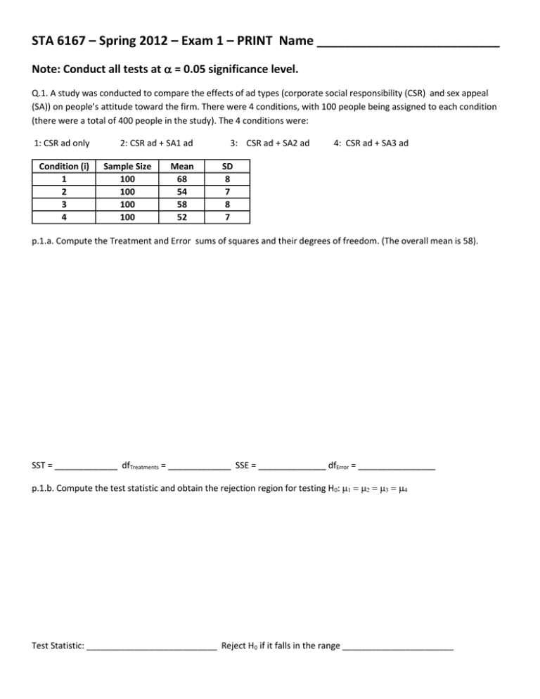
STA 6167 – Spring 2012 – Exam 1 – PRINT Name __________________________
Note: Conduct all tests at  = 0.05 significance level.
Q.1. A study was conducted to compare the effects of ad types (corporate social responsibility (CSR) and sex appeal
(SA)) on people’s attitude toward the firm. There were 4 conditions, with 100 people being assigned to each condition
(there were a total of 400 people in the study). The 4 conditions were:
1: CSR ad only
Condition (i)
1
2
3
4
2: CSR ad + SA1 ad
Sample Size
100
100
100
100
Mean
68
54
58
52
3: CSR ad + SA2 ad
4: CSR ad + SA3 ad
SD
8
7
8
7
p.1.a. Compute the Treatment and Error sums of squares and their degrees of freedom. (The overall mean is 58).
SST = _____________ dfTreatments = _____________ SSE = ______________ dfError = ________________
p.1.b. Compute the test statistic and obtain the rejection region for testing H0: 






Test Statistic: ___________________________ Reject H0 if it falls in the range _______________________
Q.2. A multiple regression model was fit, relating consumer’s satisfaction of culinary (food) event (Y) to the following
predictor variables/scales: food tasting (X1), food/beverage prices (X2), ease of coming/going to event (X3), and
convenient parking (X4). The regression model was fit, based on n=277 respondents, with R2 = 0.44. The regression
coefficients are given below, for the model: E(Y) = X1X2X3 X4
Parameter
Constant
X1
X2
X3
X4
Estimate
1.805
0.327
0.263
0.082
0.025
StdError
0.156
0.041
0.052
0.035
0.042
t
11.571
7.976
2.343
0.595
p.2.a. Test H0: Customer satisfaction is not associated with any of the predictors ( ).
p.2.a.i. Test Statistic:
p.2.a.ii. Reject H0 if the test statistic falls in the range __________________________________
p.2.b. Test H0: Controlling for all other predictors, customer satisfaction is not associated with food/bev prices (0).
p.2.b.i. Test Statistic:
p.2.b.ii. Reject H0 if the test statistic falls in the range __________________________________
Q.3. A one-way analysis of variance was conducted to compare 5 conditions in terms of respondents’ beliefs in
paranormal activity. The responses are change scores in paranormal beliefs after being exposed to a television show
about paranormal events (Positive values mean their beliefs increased, negative mean decreased. There were 22 people
in each condition (for a total N=22(5) =110) and the Within Mean Square is MSE = 16. The conditions are (based on
disclaimers prior to show):
1: Disclaimer that story in the show is based on reality, but is a re-enactment (Mean1 = -1.0)
2: Disclaimer that the story in the show is purely fiction (Mean2 = -1.6)
3: Disclaimer that the story in the show is impossible (Mean3 = -2.0)
4: No Disclaimer (Mean4 = + 1.6)
5: No story shown (comedy show shown instead) (Mean5 = -0.8)
p.3.a. Compute Bonferroni’s minimum significant difference for comparing any 2 pairs of conditions:
p.3.b. Complete the following Table (and circle correct decision for each pair, where NSD = not significantly different):
i,j
1,2
1,3
1,4
1,5
2,3
2,4
2,5
3,4
3,5
4,5
Mean(i)-Mean(j)
0.6
1
-2.6
-0.2
0.4
-3.2
-0.8
mu(i)<mu(j)
mu(i)<mu(j)
mu(i)<mu(j)
mu(i)<mu(j)
mu(i)<mu(j)
mu(i)<mu(j)
mu(i)<mu(j)
mu(i)<mu(j)
mu(i)<mu(j)
mu(i)<mu(j)
Conclude
mu(i) > mu(j)
mu(i) > mu(j)
mu(i) > mu(j)
mu(i) > mu(j)
mu(i) > mu(j)
mu(i) > mu(j)
mu(i) > mu(j)
mu(i) > mu(j)
mu(i) > mu(j)
mu(i) > mu(j)
NSD
NSD
NSD
NSD
NSD
NSD
NSD
NSD
NSD
NSD
Q.4. A linear regression model is fit, relating Y to 3 independent variables. The researcher is interested in determining
whether any interactions are significant among the 3 independent variables. She fits the following 2 models (n = 30):
Model 1: E Y     1 X 1   2 X 2   3 X 3
R12  0.48
Model 2: E Y     1 X 1   2 X 2   3 X 3   4 X 1 X 2  5 X 1 X 3   6 X 2 X 3
R22  0.54
p.4.a. Compute the test statistic for testing H0: No interactions among X1, X2, and X3 ( )
p.4.b. Reject H0 if the test statistic falls in the range ____________________________________________
Q.5. For the following scenarios, fill in the missing values.
p.5.a. Multiple linear regression, n=32 subjects, p=6 predictor variables. Testing H0:  

Numerator df = ______________
Denominator df = ______________ Rejection Region: Fobs ____________
p.5.b. 1-Way ANOVA (Completely Randomized Design), t treatments, r subjects/Trt.
Testing H0: Rejection Region: Fobs ≥ 3.490

# Treatments = t = _________________
# Replicates/Treatment = r = _______________
p.5.c. 2-Way ANOVA (Randomized Block Design), t = 3 treatments, b = 6 blocks. Bonferroni’s Minimum Significant
Difference (MSE = 300):

t.025,C,df = ______________


SE y i  y j =_________________________ Bij = __________________
Q.6. A Randomized Block Design is conducted to compare t = 3 brands of puppy chow on weight gain of puppies. Three
male puppies from 6 litters were selected, where the litters are blocks. Within litters, puppies are randomized so that
one gets brand A, one gets brand B, and one gets brand C. Data are given in the following table (where the response is
weight gain in a 3-week period). Note that the total sum of squares is: TSS = 129.28
Litter\Brand
1
2
3
4
5
6
Brand Mean
A
4.20
8.20
2.20
9.40
3.20
8.80
6.00
B
2.80
5.60
2.00
7.20
2.50
3.90
4.00
C
2.00
4.20
1.80
7.40
0.30
2.30
3.00
Litter Mean
3.00
6.00
2.00
8.00
2.00
5.00
4.33
p.6.a. Given the following quantities, complete the ANOVA table (be careful of needed multipliers).
 3  4.33   6  4.33   2  4.33  8  4.33   2  4.33  5  4.33
2
2
2
 6  4.33   4  4.33  3  4.33  4.67
2
Source
Brand (Trt)
Litter (Blk)
Error
Total
2
2
df
2
SS
129.28
2
2
 28.80
MS
F
F(0.05)
#N/A
#N/A
#N/A
#N/A
#N/A
#N/A
#N/A
Significant Effects?
Yes / No
#N/A
#N/A
#N/A
p.6.b. Conduct Friedman’s Test to determine whether there are differences among the brands on weight gain:
p.6.b.i. T1 = _________________________
T2 = _____________________ T3 = ________________________
p.6.b.ii. Test Statistic:
p.6.b.iii. Reject H0 if test statistic falls in the range _________________________________________
Q.7. All possible regressions are fit among models containing 3 potential independent variables. Complete the following
table. The models are based on n=24 observations.
Model
X1
X2
X3
X1,X2
X1,X3
X2,X3
X1,X2,X3
p'
SS(Reg)
200
300
500
400
750
SS(Res) R-square MS(Res) Adj-RSq
800
0.164
700
31.818 0.268
500
22.727 0.477
0.343
600
28.571 0.343
0.726
200
10.000 0.781
Cp
60
50
30
AIC
88.157
84.953
76.877
SBC
90.513
87.309
79.233
42
83.253
86.787
4
58.886
63.599
p.7.a. Complete the table. Note:
CP 
SS  Error Model
MS  Error Complete
 2 p ' n
AIC  n ln  SS  Error Model   2 p ' n ln(n)
SBC  BIC  n ln  SS  Error Model   ln(n) p ' n ln(n)
p.7.b. A researcher chooses the best model based on the SBC criterion. Which model will be selected? Why?
p.7.c. Another researcher chooses the best model based on CP, which model is selected? Why?