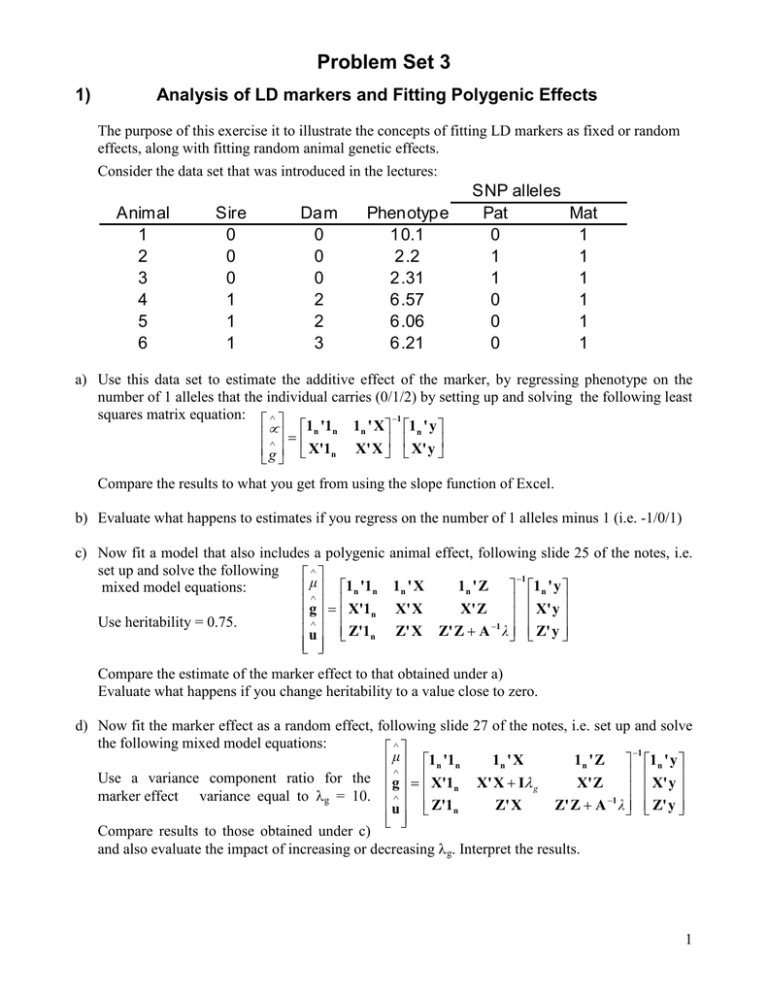
Problem Set 3
1)
Analysis of LD markers and Fitting Polygenic Effects
The purpose of this exercise it to illustrate the concepts of fitting LD markers as fixed or random
effects, along with fitting random animal genetic effects.
Consider the data set that was introduced in the lectures:
Animal
1
2
3
4
5
6
Sire
0
0
0
1
1
1
Dam
0
0
0
2
2
3
Phenotype
10.1
2.2
2.31
6.57
6.06
6.21
SNP alleles
Pat
Mat
0
1
1
1
1
1
0
1
0
1
0
1
a) Use this data set to estimate the additive effect of the marker, by regressing phenotype on the
number of 1 alleles that the individual carries (0/1/2) by setting up and solving the following least
squares matrix equation:  ∧ 
−1
1 '1 1n ' X  1n ' y 
 µ∧  =  n n
 

 g   X'1n X' X   X' y 
 
Compare the results to what you get from using the slope function of Excel.
b) Evaluate what happens to estimates if you regress on the number of 1 alleles minus 1 (i.e. -1/0/1)
c) Now fit a model that also includes a polygenic
set up and solve the following
∧
mixed model equations:
 µ∧  1n '1n
 g  =  X'1
n
∧ 
Use heritability = 0.75.

Z'1
u  
n
 
animal effect, following slide 25 of the notes, i.e.
1n ' X
1n ' Z 
X' X
X' Z 
Z' X Z' Z + A −1 λ 
−1
1n ' y 
 X' y 


 Z' y 
Compare the estimate of the marker effect to that obtained under a)
Evaluate what happens if you change heritability to a value close to zero.
d) Now fit the marker effect as a random effect, following slide 27 of the notes, i.e. set up and solve
the following mixed model equations:
∧
−1
1n ' X
1 n ' Z  1n ' y 
 µ∧  1n '1n
Use a variance component ratio for the  g  =  X'1
X' X + Iλ g
X' Z   X' y 
n



marker effect variance equal to λg = 10. ∧
Z' X
Z' Z + A −1 λ   Z' y 
u   Z'1n
 
Compare results to those obtained under c)
and also evaluate the impact of increasing or decreasing λg. Interpret the results.
1
e) Compute the EBV of each animal based on the model under c) and d) and compare results. EBV
are the sum of the estimate based on the marker (X ĝ ) and the polygenic EBV ( û ) and can be
gˆ 
computed as: [X Z ]  
uˆ 
f) Compute the accuracy of the EBV of each animal based on model d). Accuracies can be computed
based
on
the
prediction
error
variance-covariance
matrix:
C XX
PEV = [X Z] ZX
C
C XZ   X' 2
  σ e
C ZZ   Z'
where CXX is the block of the inverse of the left hand sides corresponding to X’X, etc.:
1n '1n
 X'1
n

 Z'1n
and
σ e2
1n ' X
1n ' Z 
X' X
X' Z 
Z' X Z' Z + A −1 λ 
−1
 C 11

= C X 1
 X Z1

is the environmental variance, which is equal to h
Z 1X
C XX
C ZX
C 1Z 

C XZ 
C ZZ 
σ p2 . Assume σ p2 = 9 .
2
Then, the accuracy of animal i can be computed as: ri = 1 −
PEV ( EBVi )
σ a2
Where PEV(EBVi) is the ith diagonal of the PEV matrix.
2