Section 7.3: Continuous Random Variable Applications
+
)*' (
& & &&& & &
&&&
&
&&&
&&&
&&&
&&&
&&&
&&&
&&&
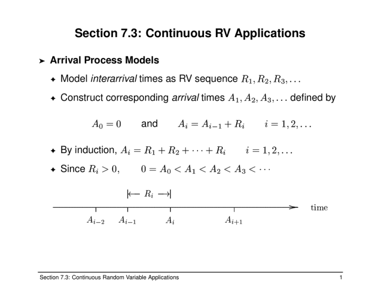
Construct corresponding arrival times
&&&
✦
Model interarrival times as RV sequence
&&&
%
✦
&&&
&&&
&&&
&&&
&&&
&&&
&&&
&&&
&&&
&&&
&&&
&&&
&&&
&&&
&&&
&&&
&&&
&&&
&&&
&&&
"
$
#"!
and
&&&
&&&
&&&
&&&
&&&
&&&
&&&
&&&
&&&
&&&
&&&
Since
✦
By induction,
&&&
&&&
&&&
&&&
&&&
&&&
&&&
&&&
&&&
&&&
&&&
✦
&&&
&&&
&&&
&&&
➤
&&&
&&&
&&&
&&&
&&&
Section 7.3: Continuous RV Applications
Arrival Process Models
defined by
1
Example 7.3.1
0
,
#
/.
Programs ssq2 and ssq3 generate job arrivals in this way, where
are Exponential
-
➤
1
jobs per unit
0
/.
Programs sis3 and sis4 generate demand instances in this way,
interdemand times
with Exponential
-
➤
/
In both programs, the arrival rate is equal to
time
2
✦
/
✦
actual demands per time interval in sis3
potential demands per time interval in sis4
/
The demand rate corresponds to an average of
Section 7.3: Continuous Random Variable Applications
2
Definition 7.3.1
Stationary arrival processes also known as
/
Renewal processes
Homogeneous arrival processes
Arrival rate
/
has units “arrivals per unit time”
If average interarrival time is
minutes,
then the arrival rate is
arrivals per minute
✦
Stationary arrival processes are “convenient fiction”
If the arrival rate
varies with time, the arrival process is
nonstationary (see Section 7.5)
/
➤
✦
➤
✦
5
34
✦
is an iid sequence of positive interarrival times with
, then the corresponding sequence of arrival times
is a stationary arrival process with rate
/. ➤
If
➤
➤
Section 7.3: Continuous Random Variable Applications
3
Stationary Poisson Arrival Process
0
/.
As in ssq2, ssq3, sis3 and sis4, with lack of information it is
usually most appropriate to assume that the interarrival times are
Exponential
-
➤
Section 7.3: Continuous Random Variable Applications
0
/.
is an Erlang
0
/ the arrival time
/.
2
Equivalently, for
random variable
-
If
is an iid sequence of Exponential
interarrival
of arrival times is
times, the corresponding sequence
a stationary Poisson arrival process with rate
➤
4
Algorithm 7.3.1
Given
and
, this algorithm generates a realization of a
stationary Poisson arrival process with rate over
/
60
6
/
➤
);
8 7
7
87
7
7
87
:
/
987
7
= 0.0; /* a convention */
n = 0;
< t)
while(
=
+ Exponential(1 /
n++;
;
return
Section 7.3: Continuous Random Variable Applications
5
Random Arrivals
In the following discussion,
defines a fixed time interval
represents the number of arrivals in the interval
is the length of a small subinterval located at random
interior to
60
;
✦
60
✦
<
✦
6
➤
We now demonstrate the interrelation between Uniform, Exponential
and Poisson random variables
60
➤
Correspondingly,
is the arrival rate
is the probability that a particular arrival will be in the
subinterval
is the expected number of arrivals in the
subinterval
<
=
✦
<
<
;
=
6
/
.
✦
;
6
.
✦
;
6
/
.
➤
Section 7.3: Continuous Random Variable Applications
6
Theorem 7.3.1
60
>
➤
that fall in
60
random
;
= 0
<
➤
=6
>
Let
be an iid sequence of Uniform
variables (“unsorted” arrivals)
Let the discrete random variable
be the number of
interior to
a fixed subinterval of length
Then is a Binomial
random variable
➤
6
<
=
;
= 0
is a Binomial
= 0
-
>
>
>
>
>
>
?
>
and
is an iid sequence of Bernoulli
8 >
Because
➤
if
is in the subinterval
otherwise
8 >
Define
➤
is in the subinterval with probability
Each
➤
.
Proof:
RVs,
,
random variable
Section 7.3: Continuous Random Variable Applications
7
Theorem 7.3.1 can be restated as Theorem 7.3.2:
for large
60
=6
;
6
/
.
<
< 0
/-
✦
;
6
>
.
<
✦
60
>
Let
be an iid sequence of Uniform
random
variables
Let the discrete random variable
be the number of
that fall
in a fixed subinterval of length
interior to
If
is large and
small,
is indistinguishable from a
random variable with
Poisson
✦
Binomial
;
/
<
.
; 0
➤
< 0
@
Recall that Poisson
/-
➤
;
Random Arrivals Produce Poisson Counts
Section 7.3: Continuous Random Variable Applications
8
Example 7.3.2
60
;
Suppose
Uniform
random variables are generated
and tallied into a continuous-data histogram with 1000 bins of size
<
6
.
➤
If bin counts are tallied into a discrete-data histogram
0
.
-
;
-
0
✦
✦
<
6
60
/
.
Since
,
from Thm 7.3.2, the relative frequencies will agree with the pdf of
random variable
a Poisson
-
➤
Section 7.3: Continuous Random Variable Applications
9
More on Random Arrivals
If many arrivals occur at random with a rate of , the number of
arrivals that will occur in an interval of length is Poisson
/-
<
>
arrivals in an interval with length
➤
The probability of no arrivals is:
➤
The probability of at least one arrival is
< 0
/
FE
HG I
/
< 0
FE
HG I
0
H 0
>
CB
>
DCB
H 0
>
CB
-
AK
A
is
< 0J
< 0
/-
A 0
>
DCB
-
/
FE
HG I
<
The probability of
A
➤
< 0
/
➤
For a fixed , the probability of at least one arrival increases with
increasing interval length
/
<
➤
Section 7.3: Continuous Random Variable Applications
10
Random Arrivals Produce Exponential Interarrivals
If represents the time between consecutive arrivals, the possible
values of are
<
➤
selected at random and an interval of
H
this interval
VWT U
X
QM L
R
<
<
< 0
H /
FE
HG I
0
0
is an Exponential
/.
DCB
-
at least one arrival
-
➤
iff there is at least one arrival in
is
^
CB
< 0
The cdf of
-
➤
QM L
P
NML
will be less than
:
➤
ODNML
P
SSS SS
SS
Z
ZZ
ZZ
[
#ZY
]
\]
Consider arrival time
length beginning at
<
➤
random variable
Section 7.3: Continuous Random Variable Applications
11
Theorem 7.3.3
If arrivals occur at random with rate , the corresponding interarrival
times form an iid sequence of Exponential
RVs
0
-
/.
/
➤
➤
➤
Proof: previous slide
Theorem 7.3.3 justifies the use of Exponential interarrival times in
programs ssq2, ssq2, sis2, sis4
If we know only that arrivals occur at random with a constant rate
, the function GetArrival in ssq2 and ssq3 is appropriate
If we know only that demand instances occur at random with a
constant rate , the function GetDemand in sis3 and sis4 is
appropriate
/
✦
/
✦
Section 7.3: Continuous Random Variable Applications
12
Generating Poisson Random Variates
Observation:
If arrivals occur at random with rate
,
the number of arrivals
in an interval of length
Poisson
random variate (Thm. 7.3.2)
lm
Example 7.3.3: an algorithm to generate a Poisson
q
p*n o
-
➤
_ 0
cga
af
cea
cda
cba
`
hh h hh h
hh
j
j
j
j
j
j
j
j
j
j
j
j
j
j
j
j
j
j
j
j
j
j
j
j
j
j
j
j
j
#ji
k
m
-
will be a
_ 0
✦
_
>
✦
/
➤
_
7
= 0.0;
x = 0;
while (a < ) {
a += Exponential(1.0);
x++;
}
return x-1;
Section 7.3: Continuous Random Variable Applications
13
Summary of Poisson Arrival Processes
Given a fixed time interval
, there are two ways of generating a
realization of a stationary Poisson arrival process with rate
/
60
➤
60
and
✦
➤
Statistically, the two approaches are equivalent
The first approach is computationally more expensive, especially
for large
;
➤
87
7
7
7
;
;
/-
Generate the number of arrivals:
Poisson
Generate a Uniform
random variate sample of size
sort to form
Use Algorithm 7.3.1
60
✦
➤
The second approach is always preferred
Section 7.3: Continuous Random Variable Applications
14
Summary of Arrival Processes
➤
The mode of the exponential distribution is 0
✦
A stationary Poisson arrival process exhibits “clustering”
0
r.
The bottom axis shows a stationary arrival process with
interarrival times
Erlang
s ss ss
ss
vwt u
x
z zz zz
zz
}w{ |
~

y
r-
➤
/
The top axis shows a stationary Poisson arrival process with
➤
➤
The stationary Poisson arrival process generalizes to
a stationary arrival process when exponential interarrival times
are replaced by any continuous RV with positive support
a nonstationary Poisson arrival process when varies over time
/
✦
✦
Section 7.3: Continuous Random Variable Applications
15
Service Process Models
No well-defined “default”, only application-dependent guidelines:
Uniform
service times are usually inappropriate since they
rarely “cut off” at a maximum value
Service times are positive, so they cannot be Normal
unless truncated to positive values
Positive probability models “with tails”, such as the Lognormal
distribution, are candidates
If service times are the sum of
iid Exponential
sub-task
model is appropriate
times, then the Erlang
-
;
€0
✦
;
€0
✦
7
€0
✦
_
 0
€
✦
7
€0
➤
Section 7.3: Continuous Random Variable Applications
16
Program ssq4
Program ssq4 is based on program ssq3, but with a more realistic
Erlang
service time model
1
20
➤
As in program ssq3, ssq4 uses Exponential
interarrivals
-
➤
0
The corresponding service rate is 2/3
random variate
The corresponding arrival rate is 1/2
Section 7.3: Continuous Random Variable Applications
17
Example 7.3.4
1
/
For both ssq3 and ssq4, the arrival rate is
rate is
and the service
„
„
‚
ƒ
2
.
➤
†
➤
The dashed line represents the Uniform
Section 7.3: Continuous Random Variable Applications
service time pdf in ssq4
0
The solid line is the Erlang
1
20
➤
‘
‡ † ”
ˆ
† ”” ” ”
”””
”””””
””””””
‡ †
ˆ
””””””
””””””
‰
”””””””
””””””
”””””
”””””
‡ Š
”””
” ””
†
””
”” ”
‡ Š
””
”
”
‰
” ””
”” ” ”
””
”
”
”
‡ ‹
”
†
”” ” ”
””
”” ”
”
‡ ‹
””
”
‰
””
”” ”
”
””
”
‡ˆŒ ” ”
† ” ””
””
””” ”
‡ˆŒ ””” ”
‰ ”””
”””
””””
‡  ””
†
†
‰
†
‰
‡ †
†
‹
‡ †
‡ †
“
‘’ 
‡ †
‰Ž
†
The distribution of service times for two programs is very different
‡ Š
➤
pdf in ssq3
18
Erlang Service Times
Ÿ
Ÿ
Ÿ
—–
£¢¡
—Ÿ
œ
™—
œŸ
¢
¤¢
••• • ••• ••
••••• • • ••• •••
•
• ••
¥W˜ •• •
Ÿ •• •
•
•
••
•••••
•
•
•
¦
• • • • • • • • • • • • • • •• • • • • • • •
•
•
§ •• •
••
•
Ÿž •• •
•• •
••••
•
• • • • • • • • • • • • • • •• •• • • •
•••••
•• ••
• ••
••• •
•• •
••
•
•
•••••
• • • • • •• • • • • • • • • •
•••
•••
•
• • •••• • •
•• •
•
Ÿž
••
• • •••• • •
•• •
•
•••
•••
•••
——–
™š˜
–œ›
™—
—œ
Some service processes can be naturally decomposed into a series
of independent “sub-processes”
œŸ
➤
➤
If sub-process times are independent, a random variate service
time can be generated by generating sub-process times and
summing
In particular, if there are sub-processes, and each service subprocesses is Exponential , then the total service time will be
and the service rate will be
Erlang
Section 7.3: Continuous Random Variable Applications
;
€
.
-
;
€0
€0
➤
The total service time is the sum of each sub-process service time
;
➤
19
¨
A 0
^>
-
and
¨
ª
to
7
€0
>
CB
A 0
Suppose we wish to restrict the possible values of
➤
is between
Section 7.3: Continuous Random Variable Applications
H 7 0
©-
©€0
H
7 0
^>
CB
€
H 0
>
7
CB
€0
7
€
and with probability
>
DCB
©€0
€0
>
H «
CB
€0
>
CB
-
€
DCB
7 0
is greater or equal to with probability
©-
➤
7 0
with probability
-
is less or equal to
7
>
➤
>
Truncation in the continuous-variable context is similar to, but
simpler than, truncation in the discrete-variable context
>
➤
be a continuous random variable with possible values
^>
➤
Let
cdf
©-
➤
>
Truncation
20
Two Cases for Truncation
>
€
If and are specified, the cdf of
can be used to determine the
left-tail, right-tail truncation probabilities
H ­0
-
H >
©€0
€0
^>
DCB
­
©
and
can be used to determine left
¬ 0
7
©
-
➤
¬
­
If and are specified, the idf of
and right truncation points
-
and
€
-
7 0
©
7 0
^>
DCB
¬
-
7
➤
Both transformations are exact
Section 7.3: Continuous Random Variable Applications
21
Example 7.3.5
1
Section 7.3: Continuous Random Variable Applications
7
r
€
„
1
0
1
-
Note: the truncated Normal
random variable has a mean
of 1.85, not 1.5, and a standard deviation of 1.07, not 2.0
➤
­
and
/*a is 0.0 */
/*b is 4.0 */
„
„
The result:
➤
= cdfNormal(1.5, 2.0, a);
= 1.0 - cdfNormal(1.5, 2.0, b);
¬
­
¬
✦
Service times are non-negative
Service times are less than 4
0
Truncate distribution so that
✦
random variable to model service times
0
➤
0
Use a Normal
-
➤
22
Constrained Inversion
­
Once and are determined, the corresponding truncated random
variate can be generated by using constrained inversion
¬
);
©
¬
u = Uniform( , 1.0 (u);
return
­
➤
Section 7.3: Continuous Random Variable Applications
23
Example 7.3.6
1
0
The idf capability in rvms can be used to generate the truncated
random variate in Example 7.3.5
Normal
-
➤
±
„
and
A
¾
½
Figure shows
²
°
¯
®
³
²
®
¼¼¼
´
¼¼¼
¼¼¼
¼¼¼
¼¼¼
¼¼¼
¼¼¼
¼¼¼
¼¼¼
¼¼ ¼
¼¼¼
¼¼¼
¼¼¼
¼ ¼¼
¼¼¼
¼¼¼
¼¼ ¼
²»
¹º
¼¼¼
¼¼¼
¼¼¼
¼¼¼
¼¼¼
¼¼¼
¼¼¼
¼¼¼
¼¼¼
¼¼¼
¼¼¼
µ
¼¼ ¼
¼ ¼¼
¼¼¼
¼¼¼
¼¼¼
¼¼¼
¼¼¼
¼ ¼¼
¼¼¼
¼¼¼
¼¼¼
¼¼¼
¼ ¼¼
¼¼
·¶¯
¸
¯
¬
­
­
¬
= 0.2266274;
= 0.1056498;
u = Uniform( , 1.0 - );
return idfNormal(1.5, 2.0, u);
Section 7.3: Continuous Random Variable Applications
24
Triangular Random Variable
The distribution is appropriate
As an alternative to truncating a “traditional” model such as
or Lognormal
Erlang
If no other data is available
;
€0
✦
✦
ÍÍ
ÍÍ
ÍÍÍ
ÍÍ
ÍÍ
ÍÍ Í
ÍÍ
ÍÍ
ÍÍÍ
ÍÍ
ÍÍÍÍÍ
ÍÍ
ÍÍÍ
ÍÍÍÍÍ
ÍÍ
ÍÍÍ
ÍÍ
ÍÍÍÍÍ
ÍÍ
ÍÍÍ
ÍÍ
ÍÍÍÍÍ
Section 7.3: Continuous Random Variable Applications
Á
À
Â
ÍÍ
Ë
ÍÍ
ÍÍÍ
ÍÍ
ÍÍÍÍÍ
ÍÍÍÍÍ
Ã
ÍÍ
ÍÍ
ÍÍÍ
ÍÍÍÍÍ
ÍÍÍÍÍ
ÍÍÍÍÍ
É
ËÌÊ Æ
ÍÍ
ÍÍÍ
ÍÍ
Í
ÍÍÍÍÍ
ÍÍ
ÍÍ Í
ÍÍÍÍÍ
ÍÍÍÍÍ
ÍÍÍÍÍ
Ç Â
È
Ä
À É
Assume that the pdf of the random variable has shape
ÅÆ
➤
7
€0
➤
Triangular
model should be considered in situations where
the finite range of possible values along with the mode is known
7
€
¿ 0
➤
25
Section 7.3: Continuous Random Variable Applications
Ð
½
Ò Ó
½^
Ð Ð
Ð
½ 0
Ò Ó
Ñ
ÐÑ
ÒÏ
Ó
A
¿
J Ï
€
¿
A^
7
ÐÑ
#ÓÏ Ð
Ñ
ÒÏ
Ø
J ÐÑ
ÑØ
ÒÏ
Õ
-
€0
-
ÒÏ
A
¿
€
¿
A^
7
Ð Ñ ÒÏ Ð Ñ J Ï
Ò Ï J #ÓÏ
ÐÑ
Ó Ñ
ÐÑ
Ñ
ÒÏ
A 0
Î
7
€
¿ 0
¿
7
€
7
€0
¨
>
, and the pdf of
¿ 0
H €
¿ 0
H7
H7
Ô 
and
,
½
7 0
¿ 0
H
H¿
-
ÒÏ
H Ö
The idf is
7 0
-
×
➤
H €
A 0
The cdf is
iff
7 0
H €
-
7
©-
>
is Triangular
H €
H €
-
➤
½ 0
©
➤
7
€
¿ 0
➤
_
Properties of the Triangular Distribution
is
26