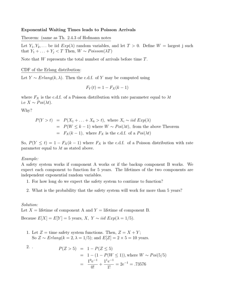
Exponential Waiting Times leads to Poisson Arrivals
Theorem: (same as Th. 2.4.3 of Hofmann notes
Let Y1 , Y2 , . . . be iid Exp(λ) random variables, and let T > 0. Define W = largest j such
that Y1 + . . . + Yj < T Then, W ∼ P oisson(λT )
Note that W represents the total number of arrivals before time T .
CDF of the Erlang distribution:
Let Y ∼ Erlang(k, λ). Then the c.d.f. of Y may be computed using
FY (t) = 1 − FX (k − 1)
where FX is the c.d.f. of a Poisson distribution with rate parameter equal to λt
i.e X ∼ P oi(λt).
Why?
P (Y > t) = P (X1 + . . . + Xk > t), where Xi ∼ iid Exp(λ)
= P (W ≤ k − 1) where W ∼ P oi(λt), from the above Theorem
= FX (k − 1), where FX is the c.d.f. of a P oi(λt)
So, P (Y ≤ t) = 1 − FX (k − 1) where FX is the c.d.f. of a Poisson distribution with rate
parameter equal to λt as stated above.
Example:
A safety system works if component A works or if the backup component B works. We
expect each component to function for 5 years. The lifetimes of the two components are
independent exponential random variables.
1. For how long do we expect the safety system to continue to function?
2. What is the probability that the safety system will work for more than 5 years?
Solution:
Let X = lifetime of component A and Y = lifetime of component B.
Because E[X] = E[Y ] = 5 years, X, Y ∼ iid Exp(λ = 1/5).
1. Let Z = time safety system functions. Then, Z = X + Y ;
So Z ∼ Erlang(k = 2, λ = 1/5); and E[Z] = 2 × 5 = 10 years.
2. .
P (Z > 5) = 1 − P (Z ≤ 5)
= 1 − (1 − P (W ≤ 1)), where W ∼ P oi(5/5)
10 e−1 11 e−1
=
+
= 2e−1 = .73576
0!
1!