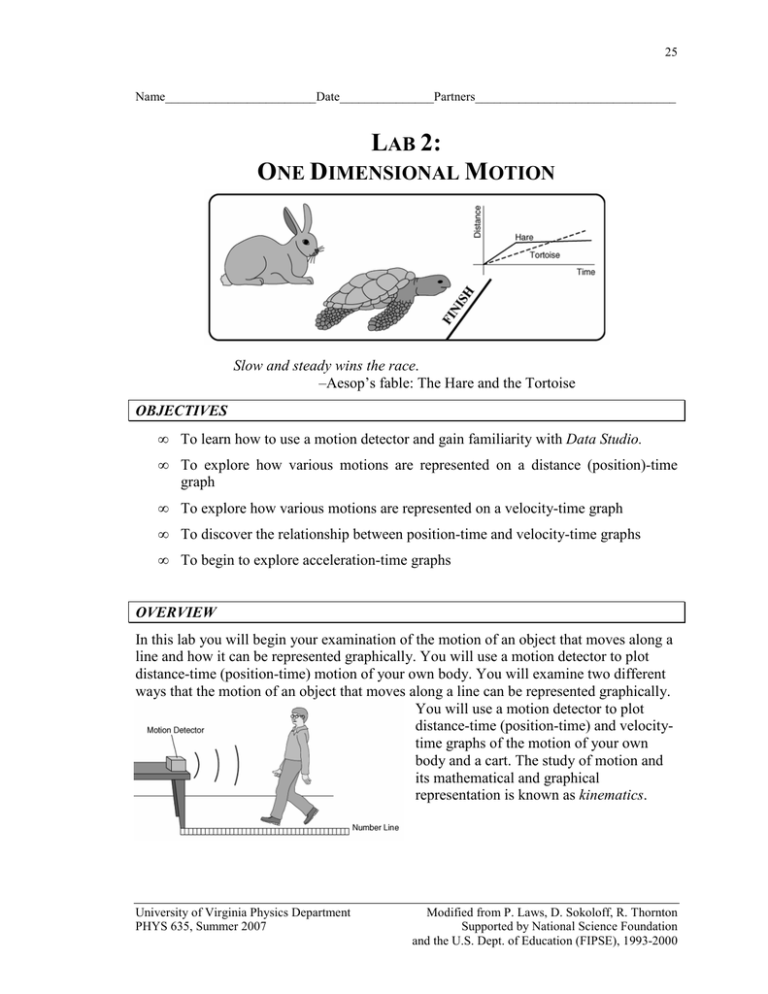
25
Name________________________Date_______________Partners________________________________
LAB 2:
ONE DIMENSIONAL MOTION
Slow and steady wins the race.
–Aesop’s fable: The Hare and the Tortoise
OBJECTIVES
•
To learn how to use a motion detector and gain familiarity with Data Studio.
•
To explore how various motions are represented on a distance (position)-time
graph
•
To explore how various motions are represented on a velocity-time graph
•
To discover the relationship between position-time and velocity-time graphs
•
To begin to explore acceleration-time graphs
OVERVIEW
In this lab you will begin your examination of the motion of an object that moves along a
line and how it can be represented graphically. You will use a motion detector to plot
distance-time (position-time) motion of your own body. You will examine two different
ways that the motion of an object that moves along a line can be represented graphically.
You will use a motion detector to plot
distance-time (position-time) and velocitytime graphs of the motion of your own
body and a cart. The study of motion and
its mathematical and graphical
representation is known as kinematics.
University of Virginia Physics Department
PHYS 635, Summer 2007
Modified from P. Laws, D. Sokoloff, R. Thornton
Supported by National Science Foundation
and the U.S. Dept. of Education (FIPSE), 1993-2000
26
Lab 2 - One Dimensional Motion
INVESTIGATION 1:
MOTION
DISTANCE (POSITION) – TIME GRAPHS OF YOUR
The purpose of this investigation is to learn how to relate graphs of distance as a function
of time to the motions they represent.
You will need the following materials:
•
motion detector
•
number line on floor in meters
Questions to consider:
How does the distance -time graph look when you move slowly? Quickly? What happens
when you move toward the motion detector? Away? After completing this investigation,
you should be able to look at a distance-time graph and describe the motion of an object.
You should also be able to look at the motion of an object and sketch a graph
representing that motion.
Comment: “Distance” is short for “distance from the motion detector.” The motion
detector is the origin from which distances are measured. The motion detector
• detects the closest object directly in front of it (including your arms if you
swing them as you walk).
• transfers information to the computer via the interface so that as you walk (or
jump, or run), the graph on the computer screen displays your distance from the
motion detector.
• will not correctly measure anything much closer than 20 cm. When making
your graphs don’t go closer than 20 cm from the motion detector.
ACTIVITY 1-1: DETERMINING THE INITIAL SPEED
1. Be sure that the interface is connected to the computer. Open Data Studio. Click on
Create Experiment on the opening page or under File, click on New Activity, which
will go to the page where you can click on Create Experiment.
2. Click on Digital Channel Input 1 on far left. A list of sensors appears. Find the
Motion Sensor line, double click on the Icon beside the Motion Sensor line, and the
software will connect the Motion Sensor to the 750 Interface. You should physically
have the Motion Detector plugged into the Interface in the same manner. Close the
Setup by clicking on the X in the upper right.
3. On the left side of the screen under Data, click on Position and drag it down to the
graph icon in the display window. A graph should appear on the right side of the
screen displaying Position vs. Time.
4. Note that you can change the scale on both axes by moving the mouse to the
numbers, click and drag them to decrease or increase the scale. Try this for both
scales.
University of Virginia Physics Department
PHYS 635, Summer 2007
Modified from P. Laws, D. Sokoloff, R. Thornton
Supported by National Science Foundation
and the U.S. Dept. of Education (FIPSE), 1993-2000
Lab 2 – One Dimensional Motion
27
5. To start the experiment, click on the Start button. Notice then that this button is
replaced by a Stop button that allows you to stop the experiment.
6. You can erase data by clicking on Experiment on the top row and then clicking on
Delete Last Data Run. Be careful of Deleting All Data if you don't mean to do so.
7. Check that the switch on the motion detector is set to broad beam.
8. Begin graphing and make distance-time graphs for different walking speeds and
directions.
a. Start at the ½ meter mark and make a distance-time graph, walking away from the
detector (origin) slowly and steadily.
b. Make a distance-time graph, walking away from the detector (origin) medium fast
and steadily.
c. Start at the 2 meter mark and make a distance-time graph, walking toward the
detector (origin) slowly and steadily.
d. Make a distance-time graph, walking toward the detector (origin) medium fast
and steadily.
e. Click on Stop when finished.
9. Print one set of graphs for your group.
Comment: If you do not erase the graph, it will remain stored in the computer so
that it is persistently displayed on the screen. You can also go to the Data icon and
click on and off this run so the data are or are not displayed.
Prediction 1-1: Predict the position-time graph produced when a person starts at the 1 m
mark, walks away from the detector slowly and steadily for 5 s, stops for 5 s, and then
walks toward the detector twice as fast. Draw your prediction on the left axes below.
Label the axes appropriately. Compare your predictions with those made by others in
your group. Draw your group’s prediction on the right-hand axes below. The individual
prediction should be done before coming to lab.
Group Prediction
Position (m)
Position (m)
Individual Prediction
Time (s)
Time (s)
10. Test your prediction by using the computer to graph your position over a range of 2 m
for a time interval of 15 s. Move in the way described in Prediction 1-1, and graph
your motion.
University of Virginia Physics Department
PHYS 635, Summer 2007
Modified from P. Laws, D. Sokoloff, R. Thornton
Supported by National Science Foundation
and the U.S. Dept. of Education (FIPSE), 1993-2000
28
Lab 2 - One Dimensional Motion
11. When you are satisfied with your graph, print one copy of the graph for your group.
Question 1-1: Is your prediction the same as the final result? If not, describe how you
would move to make a graph that looks like your prediction.
12. Everyone should gather around the computer for the next few steps to make sure
everyone learns how to do these manipulations with Data Studio.
13. Keep the previous graph of your motion on the screen. Change scales as desired or
use the Autoscale (scale to fit) icon on the Graph window toolbar on far left. Click
the Autoscale to see what happens.
14. Click on the Smart Tool and drag the crosshair to individual data points to read the
data at that point.
15. To highlight regions of data, go to a beginning spot and “click-and-drag” a window
around the region of interest. Data will be highlighted with yellow background.
Highlight the first region of data when you walk away from the motion detector.
16. To fit data, click on the Fit icon and choose the function you desire, in this case
Linear Fit. Note the parameters (slope and y-intercept) are immediately given on the
screen. To remove them, go back and “unclick” Linear Fit.
17. Note that if you leave Linear Fit on, but choose a different highlighted region, the fit
will be applied to the new region.
18. Let's now examine the region where the person was at rest. Highlight the second
region of your data which should be level. Then click on the Statistics icon (which
appears as a Σ). Click on Mean and the mean value over that region will be
displayed. Note the varying functions that can be obtained with the Statistics
functions.
19. If you have multiple runs on the screen, note that the various tools work on the run
that is highlighted in the box in yellow. You can choose which data runs are
displayed by clicking on the Data icon and clicking on and off the runs as you desire.
20. Now find the slopes of the two regions in which you were walking. Remember that
the return path was supposed to be twice as fast as the initial path. Use the Tools to
find the velocity (slope) of each path:
First path slope: _________________
University of Virginia Physics Department
PHYS 635, Summer 2007
Second path slope: __________________
Modified from P. Laws, D. Sokoloff, R. Thornton
Supported by National Science Foundation
and the U.S. Dept. of Education (FIPSE), 1993-2000
Lab 2 – One Dimensional Motion
29
Question 1-2: How did you do? Was the speed in the second path about twice that in
the first?
INVESTIGATION 2: POSITION-TIME GRAPHS OF MOTION
The purpose of this investigation is to learn how to relate graphs of position as a function
of time to the motions they represent.
You will need the following materials:
• motion detector
• number line on floor in meters
ACTIVITY 2-1: MATCHING A POSITION-TIME GRAPH
By now you should be pretty good at predicting the shape of a position-time graph of
your movements. Can you do things the other way around: reading a position-time graph
and figuring out how to move to reproduce it? In this activity you will move to match a
position graph shown on the computer screen.
Position (m)
4
3
2
1
0
0
5
10
15
20
25
Time (s)
1. In Data Studio, select “Open” and navigate to the “203” folder. Do not try to save
the previous activity (you will be prompted to do this). Open the experiment file
called L02.A2-1 Position Match. A position graph like that shown above will appear
on the screen. Clear any other data remaining from previous experiments.
Comment: This graph is stored in the computer so that it is persistently displayed
on the screen. New data from the motion detector can be collected without erasing
the Position Match graph.
2. Try to move so as to duplicate the Position Match graph on the computer screen.
You may try a number of times. It helps to work as a team. Each person should take a
turn.
University of Virginia Physics Department
PHYS 635, Summer 2007
Modified from P. Laws, D. Sokoloff, R. Thornton
Supported by National Science Foundation
and the U.S. Dept. of Education (FIPSE), 1993-2000
30
Lab 2 - One Dimensional Motion
Question 2-1: What was different in the way you moved to produce the two differently
sloped parts of the graph you just matched?
INVESTIGATION 3: VELOCITY-TIME GRAPHS OF MOTION
You have already plotted your position along a line as a function of time. Another way to
represent your motion during an interval of time is with a graph that describes how fast
and in what direction you are moving. This is a velocity-time graph. Velocity is the rate of
change of position with respect to time. It is a quantity that takes into account your speed
(how fast you are moving) and also the direction you are moving. Thus, when you
examine the motion of an object moving along a line, the direction the object is moving
is indicated by the algebraic sign (positive or negative) of the velocity.
Graphs of velocity vs. time are more challenging to create and interpret than those for
position. A good way to learn to interpret them is to create and examine velocity-time
graphs of your own body motions, as you will do in this investigation.
You will need the following materials:
• motion detector
• number line on floor in meters
ACTIVITY 3-1: MAKING VELOCITY GRAPHS
1. Open the experiment file called L02.A3-1 Velocity Graphs. This will allow you to
graph velocity. Check that the switch on the motion detector is on the broad beam.
2. You will want to walk at different speeds to match the motion as described in (a)-(d)
below. Each member of the group should try at least one of these. Ask your TA how
to choose what data are displayed on the screen (and printed out). Basically you click
on and off various runs under the DATA icon to show on the screen
a. Begin graphing and make a velocity graph by walking away from the detector
slowly and steadily. Try again until you get a graph you’re satisfied with. You
may want to adjust the velocity scale so that the graph fills more of the screen
and is clearer.
b. Make a velocity graph, walking away from the detector medium fast and steadily.
STOP the data taking after each try. Then START for the next experiment.
c. Make a new velocity graph, walking toward the detector slowly and steadily.
d. Make a new velocity graph, walking toward the detector medium fast and
steadily.
University of Virginia Physics Department
PHYS 635, Summer 2007
Modified from P. Laws, D. Sokoloff, R. Thornton
Supported by National Science Foundation
and the U.S. Dept. of Education (FIPSE), 1993-2000
Lab 2 – One Dimensional Motion
31
3. Print out one graph that includes all the data you decide to keep. Make sure you
denote on your print out with letters a) – d) to indicate what you were trying to do.
Question 3-1: What is the most important difference between the graph made by slowly
walking away from the detector and the one made by walking away more quickly?
Question 3-2: How are the velocity-time graphs different for motion away THAN FOR
motion towards the detector?
Prediction 3-1: Each person draw below in your own manual, using a dashed line, your
prediction of the velocity-time graph produced if you, in succession,
•
•
•
walk away from the detector slowly and steadily for about 5 s
then stand still for about 5 s
then walk toward the detector steadily about twice as fast as before.
Do the predictions before coming to lab. Label your predictions and compare with your
group to see if you can all agree. Use a solid line to draw in your group prediction.
Velocity (m/s)
1
0
-1
0
2.5
5
7.5
10
12.5
15
Time (s)
4. Test your prediction. (Adjust the time scale to 15 s.) Be sure to think about your
starting point! Begin graphing and repeat your motion until you think it matches the
description.
University of Virginia Physics Department
PHYS 635, Summer 2007
Modified from P. Laws, D. Sokoloff, R. Thornton
Supported by National Science Foundation
and the U.S. Dept. of Education (FIPSE), 1993-2000
32
Lab 2 - One Dimensional Motion
5. Print out one copy of the best graph for your group report.
ACTIVITY 3-2: MATCHING A VELOCITY GRAPH
In this activity, you will try to move to match a velocity-time graph shown on the
computer screen. This is much harder than matching a position graph as you did in the
previous investigation so do not spend a lot of time on this activity. Most people find it
quite a challenge to move so as to match a velocity graph. In fact, some velocity graphs
that can be invented cannot be matched!
Velocity (m/s)
1. Open the experiment file called L02.A3-2 Velocity Match to display the velocitytime graph shown below on the screen.
1
0
-1
0
4
8
12
16
20
Time (s)
Prediction 3-2: Describe in words how you would move so that your velocity matched
each part of this velocity-time graph. Do this before coming to lab.
0 to 4 s:
4 to 8 s:
8 to 12 s:
12 to 18 s:
18 to 20 s:
2. Begin graphing, and move so as to imitate this graph. Try to do this without looking
at the computer screen. You may try a few times. Work as a team and plan your
movements. Get the times right. Get the velocities right. It is quite difficult to obtain
University of Virginia Physics Department
PHYS 635, Summer 2007
Modified from P. Laws, D. Sokoloff, R. Thornton
Supported by National Science Foundation
and the U.S. Dept. of Education (FIPSE), 1993-2000
Lab 2 – One Dimensional Motion
33
smooth velocities. We have smoothed the data electronically, but your results may
still oscillate significantly. Looking at the screen for feedback can actually make
things worse.
Draw in your group’s best match on the velocity-time graph shown above. As we
stated earlier, don’t spend a lot of time trying to improve this. It is difficult!
Question 3-3: Is it possible for an object to move so that it produces an absolutely
vertical line on a velocity-time graph? Explain.
Question 3-4: Did you have to stop to avoid hitting the motion detector on your return
trip? If so, why did this happen? How would you solve the problem? If you didn’t have
to stop, why not? Does a velocity graph tell you where to start? Explain.
INVESTIGATION 4: RELATING POSITION AND VELOCITY GRAPHS
You have looked at position-time and velocity-time graphs separately. Since positiontime and velocity-time graphs are different ways to represent the same motion, it is
possible to figure out the velocity at which someone is moving by examining her/his
position-time graph. Conversely, you can also figure out how far someone has traveled
(change in position) from a velocity-time graph.
To explore the relation between position-time and velocity-time graphs, you will need
the following materials:
• motion detector
• number line on floor in meters
ACTIVITY 4-1: DETERMINING VELOCITY GRAPHS FROM POSITION GRAPHS
1. Open the experiment file called L02.A4-1 Velocity from Position to set up the axes
shown that follow. Clear any previous graphs.
Prediction 4-1: Do this before coming to lab. Determine the velocity graph from a
position graph. Carefully study the position-time graph that follows and predict the
velocity-time graph that would result from the motion. Use a dashed line to sketch what
University of Virginia Physics Department
PHYS 635, Summer 2007
Modified from P. Laws, D. Sokoloff, R. Thornton
Supported by National Science Foundation
and the U.S. Dept. of Education (FIPSE), 1993-2000
34
Lab 2 - One Dimensional Motion
Position (m)
you believe the corresponding velocity-time graph on the velocity axes will be.
4
2
0
Velocity (m/s)
2
0
1
2
3
4
5
Prediction
0
Results
-2
0
1
2
3
Time (s)
4
5
2. Test your prediction. After each person has sketched a prediction, begin graphing,
and do your group’s best to make a position graph like the one shown. Walk as
smoothly as possible.
When you have made a decent duplicate of the position graph, sketch your actual
graph over the existing position-time graph. Use a solid line to draw the actual
velocity-time graph on the velocity graph where you drew your prediction. Do not
erase your prediction or your data in the computer.
Question 4-1: How would the position graph be different if you moved faster? Slower?
Question 4-2: How would the velocity graph be different if you moved faster? Slower?
ACTIVITY 4-2: CALCULATING AVERAGE VELOCITY
In this activity, you will find an average velocity from your velocity-time graph in
Activity 4-1 and then from your position-time graph.
University of Virginia Physics Department
PHYS 635, Summer 2007
Modified from P. Laws, D. Sokoloff, R. Thornton
Supported by National Science Foundation
and the U.S. Dept. of Education (FIPSE), 1993-2000
Lab 2 – One Dimensional Motion
35
1. Here you will find your average velocity from the velocity graph that you obtained in
Activity 4-1. Choose a region where your velocity is relatively constant and pick 10
adjacent velocity values. Do not choose a region where the velocity is zero. Use
the Smart Tool in Data Studio to read values of velocity and write them in the table
below. Use these values to calculate the average (mean) velocity using a calculator.
For reference, note the time at the first and last points. You will need them later.
Time at first point______________
Time at last point _________________
Velocity values (m/s)
1
6
2
7
3
8
4
9
5
10
Average (mean) value of the velocity: _______________ m/s
Comment: Average velocity during a particular time interval can also be calculated as
the change in position divided by the change in time. (The change in position is often
called the displacement.) For motion with a constant velocity, this is also the slope of
the position-time graph for that time period.
As you have observed, the faster you move, the steeper your position-time graph
becomes. The slope of a position-time graph is a quantitative measure of this incline.
The size of this number tells you the speed, and the sign tells you the direction.
2. Calculate your average velocity from the slope of your position graph in Activity 4-1.
Make sure you use the same time region here that you just used in step 1. Use the
Smart Tool again to read the position and time coordinates corresponding to the two
end points (of your ten-point velocity region).
Position (m)
Time (s)
Point 1
Point 2
3. Calculate the change in position (displacement) between points 1 and 2. Also calculate
the corresponding change in time (time interval). Divide the change in position by the
change in time to calculate the average velocity. Show your calculations below.
University of Virginia Physics Department
PHYS 635, Summer 2007
Modified from P. Laws, D. Sokoloff, R. Thornton
Supported by National Science Foundation
and the U.S. Dept. of Education (FIPSE), 1993-2000
36
Lab 2 - One Dimensional Motion
Change in position (m)
Time interval (s)
Average velocity (m/s)
Question 4-3: Does the average velocity you just calculated from the position graph
agree with the average velocity you found from the velocity graph? Do you expect them
to agree? How would you account for any differences?
ACTIVITY 4-3: USING STATISTICS AND FIT TO FIND THE AVERAGE VELOCITY
In Activity 4-2, you found the value of the average velocity for a steady motion in two
ways: from the average of a number of values on a velocity-time graph and from the
slope of the position-time graph. The statistics feature in Data Studio (look for the Σ
icon) allows you to find the average (mean) value directly from the velocity-time graph.
The fit routine should allow you to find the line that best fits your position-time graph
from Activity 4-1. The equation of this line includes a value for the slope.
1. Using statistics: You must first select the portion of the velocity-time graph for
which you want to find the mean value. Make sure you select the same region here
that you used in step 1 of Activity 4-2. Next use the statistics feature Σ to read the
mean value of velocity during this portion of the motion.
Average (mean) value of the velocity: ______________ m/s
Question 4-4: Compare this method to the one in Activity 4-2 (step 1) where you
determined the average by hand. Which method is easiest? Why?
2. Using fit: You must first select the portion of the position-time graph that you want
to fit. Use the same 10-point region you have been using.
Next, use the fit routine, select a linear fit, y = mx + b, and then find the equation of
the line.
University of Virginia Physics Department
PHYS 635, Summer 2007
Modified from P. Laws, D. Sokoloff, R. Thornton
Supported by National Science Foundation
and the U.S. Dept. of Education (FIPSE), 1993-2000
Lab 2 – One Dimensional Motion
37
Record the equation of the fit line below, and compare the value of the slope (m) to
the velocity you found in Activity 4-2.
Question 4-5: What does b represent?
ACTIVITY 4-4: PREDICTING POSITION GRAPHS FROM VELOCITY GRAPHS
Prediction 4-2: Carefully study the velocity graph shown above. Using a dashed line,
sketch your prediction of the corresponding position graph below. (Assume that you
started at the 1 m mark.)
PREDICTION AND FINAL RESULT
4
Prediction _ _ _
Results ____
3
2
1
0
0
1
2 Time (s) 3
4
5
Test your prediction.
1. First shut off the analysis features (fits and statistics), and adjust the time axis to 0
to 5 s as needed before you start.
University of Virginia Physics Department
PHYS 635, Summer 2007
Modified from P. Laws, D. Sokoloff, R. Thornton
Supported by National Science Foundation
and the U.S. Dept. of Education (FIPSE), 1993-2000
38
Lab 2 - One Dimensional Motion
2. After each person has sketched a prediction, your group should try to duplicate the
velocity-time graph by walking. Try to do it without looking at the computer monitor.
When you have made a good duplicate of the velocity-time graph, draw your actual
result over the existing velocity-time graph.
3. Use a solid line to draw the actual position-time graph on the same axes with your
prediction. (Do not erase your prediction.)
Question 4-6: How can you tell from a velocity-time graph that the moving object has
changed direction? What is the velocity at the moment the direction changes?
Question 4-7: How can you tell from a position-time graph that your motion is steady
(motion at a constant velocity)?
Question 4-8: How can you tell from a velocity-time graph that your motion is steady
(constant velocity)?
INVESTIGATION 5: INTRODUCTION TO ACCELERATION
There is a third quantity besides position and velocity that is used to describe the motion
of an object: acceleration. Acceleration is defined as the rate of change of velocity with
respect to time (just like velocity is defined as the rate of change of position with respect
to time). In this investigation you will begin to examine the acceleration of objects.
Because of the jerky nature of the motion of your body, the acceleration graphs are
erratic. It will be easier to examine the motion of a cart. In this investigation you will
examine the cart moving with a constant (steady) velocity. Later, in Lab 3 you will
examine the acceleration of more complex motions of the cart. You will need the
following:
• motion cart without friction pad
• 2-m motion track
• Level
• motion detector
University of Virginia Physics Department
PHYS 635, Summer 2007
Modified from P. Laws, D. Sokoloff, R. Thornton
Supported by National Science Foundation
and the U.S. Dept. of Education (FIPSE), 1993-2000
Lab 2 – One Dimensional Motion
39
ACTIVITY 5-1: MOTION OF A CART AT A CONSTANT VELOCITY
To graph the motion of a cart at a constant velocity you can give the cart a quick push
with your hand and then release it.
1. Clip the motion detector on the end of the ramp. Ask your TA for help if it is not
clear how to do this. Set switch to narrow beam. Be sure that the track is level.
20 cm
2. Open the experiment file called L02.A5-1 Constant Velocity.
Prediction 5-1: Do this before coming to lab. Based on your observations of the
motions of your body, how should the position and velocity graphs look if you move the
cart at a constant velocity away from the motion detector starting at the 0.3-m mark?
Sketch your predictions with dashed lines on the axes that follow.
2
1
0
1
0
-1
0
1
2
Time (s)
3
4
5
3. Test your prediction. Give the cart a quick push and release it. Be sure that the cart
is never closer than 20 cm from the motion detector and that your hand is not
between the cart and motion detector. Begin graphing right after releasing the
cart. Try several times until you get a fairly constant velocity. Sketch your results
with solid lines on the axes.
4. Print out one copy for your group report.
University of Virginia Physics Department
PHYS 635, Summer 2007
Modified from P. Laws, D. Sokoloff, R. Thornton
Supported by National Science Foundation
and the U.S. Dept. of Education (FIPSE), 1993-2000
40
Lab 2 - One Dimensional Motion
Question 5-1: Did your position-time and velocity-time graphs agree with your
predictions? Discuss. What type of curve characterizes constant velocity on a positiontime graph?
ACTIVITY 5-2: ACCELERATION OF A CART MOVING AT A CONSTANT VELOCITY
Prediction 5-2: Do this before coming to lab. Sketch with a dashed line on the axes that
follow your prediction of the acceleration of the cart you just observed moving at a
constant velocity away from the motion detector. Base your prediction on the definition
of acceleration.
PREDICTION AND FINAL RESULTS
Acceleration (m/s2)
1
0
-1
0
1
2
Time (s)
3
4
5
4. You will use the data you took in the previous activity. Display the real acceleration
graph of the cart by “dragging” acceleration data from the left column onto existing
graph. Sketch the acceleration graph using a solid line on the axes above. Ask your
TA for help if needed.
5. Print out one copy of the graph for your group report. Label it.
Question 5-2: Does the acceleration-time graph you observed agree with your
prediction? Discuss.
6. Find the average acceleration of the car using one of the techniques that you used
earlier to find the average velocity. Show your work.
University of Virginia Physics Department
PHYS 635, Summer 2007
Modified from P. Laws, D. Sokoloff, R. Thornton
Supported by National Science Foundation
and the U.S. Dept. of Education (FIPSE), 1993-2000