Proceedings of the Twenty-Sixth International Florida Artificial Intelligence Research Society Conference
Two-Stage Second Order Training in Feedforward Neural Networks
Melvin D. Robinson and Michael T. Manry
Department of Electrical Engineering
University of Texas at Arlington
woi (1, 1)
Abstract
In this paper, we develop and demonstrate a new 2nd
order two-stage algorithm called OWO-Newton. First,
two-stage algorithms are motivated and the Gauss Newton input weight Hessian matrix is developed. Block
coordinate descent is used to apply Newton’s algorithm
alternately to the input and output weights. Its performance is comparable to Levenberg-Marquardt and it
has the advantage of reduced computational complexity. The algorithm is shown to have a form of affine
invariance.
1
Op (1)
np (1)
xp (1)
yp (1)
xp (2)
yp (2)
..
.
xp (N )
Introduction
np (Nh )
The multilayer perceptron (MLP) is the most widely used
type of neural network(Shepherd 1997). Training a MLP
involves solving a non-convex optimization problem to calculate the network’s weights. The single hidden layer MLP
is the focus of our work because any continuous function
can be approximated to arbitrary precision(Cybenko 1992).
Though one-step methods such as backpropagation (Werbos 1974), conjugate gradient (Charalambous 1992) and
Levenberg-Marquardt (Hagan and Menhaj 1994) are popular, a MLP can sometimes be trained effectively using two
step methods in which not all weights are updated simultaneously. Example two-step methods include cascade correlation (Fahlman and Lebiere 1990), OWO-HWO (Chen,
Manry, and Chandrasekaran 1999) and layer by layer (Li,
Li, and Wang 2011).
Second order methods have better convergence than first
order methods; however, we must use care when employing
them because the full network Hessian is inherently rank deficient (Smagt and Hirzinger 1998) and this can create problems in training (LeCun et al. 1998). Two-step methods allow us to mitigate this problem.
In this work we combine two-step feedforward training
with 2nd -order optimization methods. This allows us to
achieve fast convergence and reduced computational complexity over one-step 2nd -order methods.
In Section 2 we briefly review MLP architecture and our
notation. Section 3 reviews the Output Weight Optimization and Newton algorithms. In Section 4 we motivate two-
..
.
..
.
yp (M )
Op (Nh )
woi (M, N )
Input layer
Hidden layer
Output layer [t]
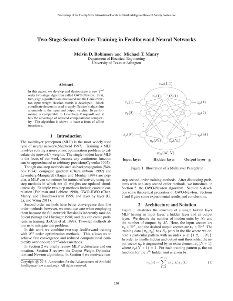
Figure 1: Illustration of a Multilayer Perceptron
step second-order training methods. After discussing problems with one-step second order methods, we introduce, in
Section 5, the OWO-Newton algorithm. Section 6 develops some theoretical properties of OWO-Newton. Sections
7 and 8 give some experimental results and conclusions.
2
Architecture and Notation
Figure 1 illustrates the structure of a single hidden layer
MLP having an input layer, a hidden layer and an output
layer. We denote the number of hidden units by Nh and
the number of outputs by M . Here, the input vectors are
xp ∈ RN , and the desired output vectors are tp ∈ RM . The
training data {xp , tp } has Nv pairs in the file where we denote a particular pattern with an index p ∈ {1, 2, . . . Nv }.
In order to handle hidden and output unit thresholds, the input vector xp is augmented by an extra element xp (N + 1),
where xp (N + 1) = 1. For each training pattern p, the net
function for the j th hidden unit is given by:
c 2013, Association for the Advancement of Artificial
Copyright Intelligence (www.aaai.org). All rights reserved.
np (j) =
N
+1
X
k=1
130
w(j, k)xp (k)
(1)
Newton’s Algorithm
so the net vector is
np = Wxp
(2)
where W is Nh by N + 1 and the corresponding hidden unit
activation Op (j) = f (np (j)). Putting everything together,
the ith output for the pth training pattern is
yp (i) =
N
+1
X
woi (i, j)xp (j) +
j=1
Nh
X
woh (i, k)Op (k)
Newton’s algorithm is the basis of a number of popular
second order optimization algorithms including LevenbergMarquardt (Levenberg 1944) and BFGS (Nocedal and
Wright 2006). Newton’s algorithm is iterative where each
iteration
• Calculates the Newton direction d
• Updates variables with direction d
The direction vector d is calculated by solving the linear
equations
Hd = g
(7)
where H is the Hessian of the objective function and g is
the gradient of the objective function as defined earlier. The
variables are then updated as
w ←w+d
(8)
Non-quadratic objective functions require a line search. This
results in w being updated as w ← w + zd.
For fast convergence we would like to use Newton’s
method to train our MLP, but the Hessian for the whole
network is singular (Wille 1997). An alternative to overcome this problem is to modify the Hessian matrix as in
the Levenberg-Marquardt algorithm. Another alternative
is to use two-step methods such as layer by layer training
(Lengellé and Denoeux 1996).
(3)
k=1
or in matrix-vector notation
yp = Woi xp + Woh Op
(4)
where Woi ∈ RM ×(N +1) , contains bypass weights, Woh ∈
RM ×Nh contains weights from hidden units to the outputs
and Op is a vector of length Nh . Some quantities that
we define for convenience are the number of input weights
Niw = Nh (N + 1), the number of network weights Nw =
Nh (N + 1) + M · Nh , and the number of basis functions
Nu = N + Nh + 1. Sometimes we refer to Woh and Woi
as wo since they are both connected to the outputs, in particular wo = vec(Woi : Woh ) where the vec() operator
concatenates matrices into a vector column by column.
3
Neural Network Training
In neural network training we choose network weights to
minimize an objective function such as the mean square error (MSE) denoted as E(w), which we will often abbreviate
as E. The MSE over a training set, called the training error,
is given by
E=
Nv X
M
1 X
2
[tp (i) − yp (i)]
Nv p=1 i=1
4
(5)
where yp (i) is given in (3) and w is a vector of network
weights, w = vec(W, Woh , Woi ).
Output Weight Optimization
One method used to train and initialize neural networks
is the Output Weight Optimization algorithm (Manry et
al. 1992). OWO calculates the output weight matrices
Woh and Woi after the input weight matrix, W is determined in some fashion, usually by random initialization.
OWO minimizes the error function
E(wo ) = woT Rwo − 2woT C + Et
Motivation for Two-Step Methods
In this section we investigate the assumptions used by Newton’s method. Newton’s method is derived from a 2nd -order
Taylor series approximation to an objective function (Boyd
and Vandenberghe 2004). Applying this principle to (5)
gives us
1
EH (w) = E0 + (w − w̃)T g + (w − w̃)T H(w − w̃) (9)
2
where w̃ is w from the previous iteration.
When applied to the MSE given in (5), Newton’s algorithm assumes that
(A1) E is approximately quadratic in w for small weight
changes
(A2) yp (i) is well approximated as a first degree function of
w.
Note that (A2) follows immediately from (A1). We investigate whether (A2) is a valid assumption by constructing a
low degree model for yp (i). A model that yields the same
Hessian and gradient as E is
(6)
In equation (6) R ∈ RNu ×Nu , C ∈ RNu ×M , and Et is
sum of average squares of the target vector elements. R
and C are estimates for the auto- and crosscorrelations of
the underlying random process. Equation (6) is minimized
by the solution to the linear equations RW = C. These
equations can be solved using any number of methods, but
special care must be taken when R is ill-conditioned. In
our work we use orthogonal least squares (Chen, Billings,
and Luo 1989). Because (6) is quadratic, OWO is merely
Newton’s algorithm for the output weights. A modern descendant of OWO is the Extreme Learning Machine (ELM)
(Huang, Zhu, and Siew 2006) training.
Ẽ =
Nv X
M
1 X
[tp (i) − ỹp (i)]2
Nv p=1 i=1
(10)
where ỹp (i) is
ỹp (i) =
N
+1
X
woi (i, n)xp (n)+
n=1
Nh
X
k=1
131
woh (i, k) Op (k) + Op0 (k)(np (k) − ñp (k))
(11)
Calculations for Input Weights
where
Op0 (k) =
ñp (k) =
∂Op (k)
,
∂np (k)
N
+1
X
w̃(k, n)xp (n)
To derive OWO-Newton we first calculate the partial derivative of E with respect to the input weights. The elements of
the negative input weight gradient matrix G ∈ RNh ×(N +1)
are given by:
(12)
(13)
n=1
g(j, k) = −
Here, w̃(k, n) = w(k, n) but w̃(k, n) is fixed in the current iteration. We have used a first order Taylor series for
each hidden unit for each pattern in the training file. Since
we have a different model ỹp (i) for each pattern, which
is first degree in xp , we can term ỹp (i) a piecewise linear
model of yp (i).
The validity of the piecewise linear model is demonstrated
by,
∂E
∂ Ẽ
=
(14)
∂w(u, v)
∂w(u, v)
and
∂2E
∂ 2 Ẽ
=
∂w(u, v)∂w(m, j)
∂w(u, v)∂w(m, j)
=
(18)
Next we calculate the Gauss-Newton input weight Hessian
denoted as HR ∈ RNiw ×Niw . Elements of HR are found as
Nv X
M
∂2E
2 X
∂yp (i) ∂yp (i)
=
∂w(j, k)∂w(l, m)
Nv p=1 i=1 ∂w(j, k) ∂w(l, m)
(15)
(19)
We use orthogonal least squares to solve
HR d = g
(20)
for d and update the input weight matrix W as
(16)
W ← W + zD
(21)
where g = vec(G) and d = vec(D). Note that in an implementation, the calculations for HR should be performed
after a lexicographic ordering of W.
In (21), z is the learning factor resulting from a line
search. A line search is necessary for OWO-Newton because
(5) is not a quadratic function of w.
When the vector w includes all the network weights contained in W, Woh , and Woi , yp (i) is a not a first order
function of the weights w. To show this, we note that the
exact expression for output vector ỹp for our network is
y˜p = Woi + Woh diag(O0p )W xp
(17)
0
+ Woh Op − diag(Op )ñp
OWO-Newton Algorithm
Require: MAXITERS > 0
Initialize W
for k=1 to MAXITERS do
Perform OWO
Calculate G
g ← vec(G)
Calculate HR
Solve (20) for d
D = vec−1 (d) as
z ← arg min E(W + zD)
The model output ỹp (i) has products woh (i, k)w(k, n). If
all network weights vary then ỹp (i) is second degree in the
unknowns and Ẽ is a fourth degree model in w and assumptions (A1) and (A2) are violated. Clearly there is a
discrepancy between Ẽ in (10) and (9). Since the products
woh (i, k)w(k, n) cause this discrepancy, the corresponding
cross terms in the network Hessian H are sources of error in
training a MLP using Newton’s method. On the other hand,
if w contains weights from only one layer, the cross terms
in (17) are first degree and the discrepancy vanishes as seen
in the input weight case in (14) and (15).
This analysis justifies the use of two-step methods where
in each iteration we fix wo and train W for one half iteration
and fix W and train wo for the other. The approach above
is called block coordinate descent (BCD) (Tseng 2001).
5
Nv X
M
2 X
∂yp (i)
[tp (i) − yp (i)]
Nv p=1 i=1
∂w(j, k)
∂yp (i)
= woh (i, j)Op0 (j)xp (k)
∂w(j, k)
Also the corresponding errors for each model, tp (i) − yp (i)
and tp (i) − ỹp (i) are equal for np (k) = ñp (k) since
∂yp (i)
= woh (i, j)Op0 (u)xp (v)
∂w(u, v)
∂ ỹp (i)
=
∂w(u, v)
∂E
∂w(j, k)
z
W ← W + zD
end for
Computational Burden
When analyzing the computational complexity of one iteration of OWO-Newton we must first run OWO to train the
output weights which requires
Nu
Mowo = Nv (Nu + 1) M +
(22)
2
OWO-Newton
One BCD approach for MLP training is to use Newton’s algorithm separately for input and output weights. Note that
Newton’s algorithm for output weights is OWO.
132
multiplies. Next, we calculate the the input weight Hessian
which requires
M (N + 1)(N + 2)
3
+
(23)
MH =Nv Niw Niw +
2
2
Proof. OWO is Newton’s method for the output weights
and Newton’s algorithm is used to train the input weights.
Therefore by Definition 1 there exist matrices TOW O and
TN ewton . As a result, we can construct a sparse T for the
entire algorithm as


..
0

TOW O .
··· 
T=

 ···
..
0
. TN ewton
multiplies. Then we must solve the linear equations to calculate the Newton direction which requires
Niw (Niw + 1)
3
Mols = Niw (Niw + 1) M +
+
(24)
6
2
The existence and sparsity of this T shows that OWONewton is partially affine invariant.
multiplies. Putting this together, the number of multiplies
required for one iteration of OWO-Newton is
MOW O−N ewton = Mowo + MH + Mols
6
Lemma 4. Partially affine invariant algorithms satisfy
Lemma 1.
(25)
Proof. The proof is the same as that of Lemma 1.
Analysis
When two equivalent networks are trained with OWONewton Ek = Ẽk for k ≥ 1 because it is partially affine
invariant.
OWO-Newton has a number of interesting properties, but
first we lay the groundwork by defining affine invariance in
a neural network training algorithm.
7
Definition 1. If two equivalent networks are formed whose
objective functions satisfy E(w) = E(Tw0 ) with w =
Tw0 , and an iteration of an optimization method yields w =
w+d and w0 = w0 +d0 where w and w0 are n-dimensional,
the training method is affine invariant if d = Td0 for every
nonsingular matrix T.
Experimental Results
In this section we compare the performance of OWONewton to LM and CG using 10-fold training and validation. For each fold, all algorithms train a MLP of a given
topology from the same initial set of weights.
Wine Data File
An algorithm lacks affine invariance if its T matrix is
constrained to be sparse. Affine invariance leads us to the
following observation of the training error sequence Ek of
equivalent networks.
We demonstrate OWO-Newton on the wine quality UCI
dataset (Frank and Asuncion 2010). The goal is to predict
the quality of wine from objective measures (Cortez et al.
2009). The training file consists of 11 features, and 1 target
(scored from 0-12) with 4898 training patterns. We train an
MLP with 15 hidden units for 200 iterations. The 10-fold
training error results are shown in Table 1. On the wine
dataset, the training error of OWO-Newton is superior to
that of LM and CG; however, the validation error for LM
is slightly better. Figure 2 illustrates the computational burden for this training characteristic.
Lemma 1. Suppose two equivalent networks initially satisfy
w = Tw0 where T is any nonsingular n × n matrix and
w is n × 1. If the training algorithm is affine invariant,
the error sequences of the two networks, Ek and Ẽk , for
iteration numbers k ≥ 1 satisfy Ek = Ẽk .
Proof. Affine invariant training of equivalent networks
yields w0 + d0 and T(w0 + d0 ) = w + d, so the networks
remain equivalent after one or more iterations.
Remote Sensing Data File
We now demonstrate OWO-Newton on the IPNNL remote
sensing dataset (Manry 1982). The goal is to predict certain
measurements related to electromagnetic scattering such as
surface permittivity, normalized surface rms roughness and
surface correlation length (Dawson, Fung, and Manry 1993).
The training file consists of 8 features and 7 targets with
1768 training patterns. We train a MLP with 10 hidden units
for 250 iterations. Table 1 shows the results of the 10-fold
training and validation error. The training error of LM is
slightly better than OWO-Newton in this example.
Lemma 2. In OWO-Newton input and output weight training is affine invariant.
Proof. In OWO-Newton, Newton’s algorithm is used for input weight training; OWO is Newton’s algorithm for output
weight training.
In multistep algorithms we train subsets of weights so we
need to define an appropriate type of affine invariance for
this case.
Prognostics Data File
Definition 2. If a training algorithm satisfies the conditions
in Definition 1 except that T is always sparse, it is partially
affine invariant.
Finally, we demonstrate OWO-Newton on a prognostics
dataset which can be obtained from the IPNNL at the University of Texas at Arlington(Manry 1982). The prognostics
training file contains parameters that are available in a helicopter’s health usage monitoring system (HUMS)(Manry,
Lemma 3. The OWO-Newton algorithm is partially affine
invariant.
133
0.56
0.54
0.25
0.52
E
E
0.5
0.2
0.48
CG
OWO-Newton
LM
0.46
0.44
0.15
0.42
CG
OWO-Newton
LM
0.1
107
108
109
1010
1011
106
Cumulative Multiplies
107
108
109
1010
Cumulative Multiplies
Figure 2: 10-fold training in the Wine dataset
Figure 3: 10-fold training in the Remote Sensing dataset
Hsieh, and Chandrasekaran 1999). It consists of topology of
17 feature vectors and 9 target vectors. The dataset consists
of 4745 training patterns. We train a MLP with 15 hidden
units for 100 iterations. Table 1 shows that OWO-Newton
trains and validates much better than LM and CG. Figure 4
shows that it accomplishes this at much less of a computational cost.
Chen, H.-H.; Manry, M. T.; and Chandrasekaran, H. 1999.
A neural network training algorithm utilizing multiple sets
of linear equations. Neurocomputing 25(1-3):55 – 72.
Cortez, P.; Cerdeira, A.; Almeida, F.; Matos, T.; and Reis,
J. 2009. Modeling wine preferences by data mining
from physicochemical properties. Decision Support Systems
47(4):547–553.
Cybenko, G. 1992. Approximation by superpositions of a
sigmoidal function. Mathematics of Control, Signals, and
Systems (MCSS) 5:455–455.
Dawson, M.; Fung, A.; and Manry, M. 1993. Surface parameter retrieval using fast learning neural networks. Remote Sensing Reviews 7(1):1–18.
Fahlman, S. E., and Lebiere, C. 1990. The cascadecorrelation learning architecture. In Advances in Neural Information Processing Systems 2, 524–532. Morgan Kaufmann.
Frank, A., and Asuncion, A. 2010. UCI machine learning
repository. http://archive.ics.uci.edu/ml.
Hagan, M., and Menhaj, M. 1994. Training feedforward
networks with the marquardt algorithm. Neural Networks,
IEEE Transactions on 5(6):989–993.
Huang, G.-B.; Zhu, Q.-Y.; and Siew, C.-K. 2006. Extreme
learning machine: theory and applications. Neurocomputing
70(1):489–501.
LeCun, Y.; Bottou, L.; Orr, G.; and Müller, K. 1998. Efficient backprop. In Orr, G., and Müller, K.-R., eds., Neural Networks: Tricks of the Trade, volume 1524 of Lecture
Notes in Computer Science. Springer Berlin / Heidelberg.
546–546.
Lengellé, R., and Denoeux, T. 1996. Training MLPs layer by
layer using an objective function for internal representations.
Neural Networks 9(1):83–97.
8
Conclusions
In this paper, we have used a piecewise linear network
model, implied by Newton’s algorithm, to motivate two-step
second order training or Block Coordinate Descent. When
Newton’s algorithm is used in both BCD steps we have the
OWO-Newton algorithm. Simulations show that the new algorithm is a good alternative to the Levenberg-Marquardt
algorithm. We have demonstrated that OWO-Newton has
fast convergence with fewer multiplies for a given error level
than LM. However we find that OWO-Newton is not guaranteed to produce a smaller validation error than LM, but that
the generalization properties are good.
Finally, we have defined affine invariance in neural networks and introduced a new property called partial affine
invariance. Analysis of OWO-Newton shows that the algorithm partially affine invariant.
References
Boyd, S., and Vandenberghe, L. 2004. Convex Optimization.
New York, NY, USA: Cambridge University Press.
Charalambous, C. 1992. Conjugate gradient algorithm for
efficient training of artificial neural networks. Circuits, Devices and Systems, IEE Proceedings G 139(3):301 –310.
Chen, S.; Billings, S.; and Luo, W. 1989. Orthogonal least
squares methods and their application to non-linear system
identification. International Journal of Control 50(5):1873–
1896.
134
Prognostics
Twod
Wine
OWO-Newton
Training Error Validation Error
Training Error
1.18314 · 107
0.125447
0.422416
1.30229 · 108
0.27557
0.511704
1.38424 · 107
0.14454
0.517243
CG
Validation Error
Training Error
1.33078 · 108
0.284679
0.53738
3.41 · 107
0.1124
0.484221
LM
Validation Error
3.67 · 107
0.137521
0.523013
Table 1: 10-fold Training and Validation Error Summary
Networks. Secaucus, NJ, USA: Springer-Verlag New York,
Inc., 1st edition.
Smagt, P. P. v. d., and Hirzinger, G. 1998. Solving the
ill-conditioning in neural network learning. In Neural Networks: Tricks of the Trade, this book is an outgrowth of
a 1996 NIPS workshop, 193–206. London, UK: SpringerVerlag.
Tseng, P. 2001. Convergence of a block coordinate descent
method for nondifferentiable minimization. J. Optim. Theory Appl. 109(3):475–494.
Werbos, P. 1974. Beyond Regression: New Tools for Prediction and Analysis in the Behavioral Sciences. Ph.D. Dissertation, Harvard University, Cambridge, MA.
Wille, J. 1997. On the structure of the Hessian matrix in
feedforward networks and second derivative methods. In
Neural Networks,1997., International Conference on, volume 3, 1851 –1855 vol.3.
E(M illions)
150
100
50
CG
OWO-Newton
LM
0
107
108
109
1010
1011
Cumulative Multiplies
Figure 4: 10-fold training in the Prognostics dataset
Levenberg, K. 1944. A method for the solution of certain
non-linear problems in least squares. Quarterly Journal of
Applied Mathematics II(2):164–168.
Li, Y.; Li, T.; and Wang, K. 2011. A new layer by layer training algorithm for multilayer feedforward neural networks.
In Advanced Computer Control (ICACC), 2011 3rd International Conference on, 600–603. IEEE.
Manry, M.; Guan, X.; Apollo, S.; Allen, L.; Lyle, W.; and
Gong, W. 1992. Output weight optimization for the multilayer perceptron. In Signals, Systems and Computers, 1992.
1992 Conference Record of The Twenty-Sixth Asilomar Conference on, 502–506. IEEE.
Manry, M.; Hsieh, C.; and Chandrasekaran, H. 1999. Nearoptimal flight load synthesis using neural nets. In Neural
Networks for Signal Processing IX, 1999. Proceedings of the
1999 IEEE Signal Processing Society Workshop., 535–544.
IEEE.
Manry, M. T. 1982. Image Processing and Neural Network
Laboratory. http://www-ee.uta.edu/eeweb/ip/new training.
html.
Nocedal, J., and Wright, S. 2006. Numerical Optimization.
Springer Verlag.
Shepherd, A. J. 1997. Second-Order Methods for Neural
135