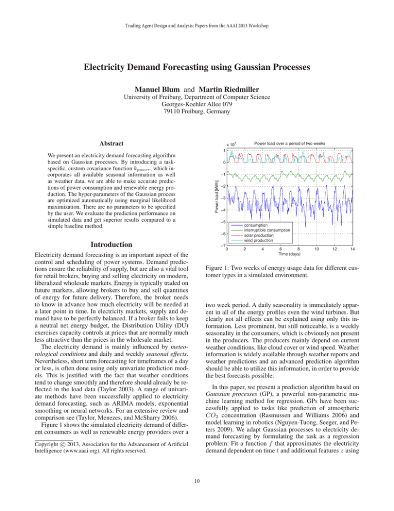
Trading Agent Design and Analysis: Papers from the AAAI 2013 Workshop
Electricity Demand Forecasting using Gaussian Processes
Manuel Blum and Martin Riedmiller
University of Freiburg, Department of Computer Science
Georges-Koehler Allee 079
79110 Freiburg, Germany
Abstract
4
Power load over a period of two weeks
x 10
1
We present an electricity demand forecasting algorithm
based on Gaussian processes. By introducing a taskspecific, custom covariance function kpower , which incorporates all available seasonal information as well
as weather data, we are able to make accurate predictions of power consumption and renewable energy production. The hyper-parameters of the Gaussian process
are optimized automatically using marginal likelihood
maximization. There are no parameters to be specified
by the user. We evaluate the prediction performance on
simulated data and get superior results compared to a
simple baseline method.
0
Power load [kWh]
−1
−2
−3
−4
−5
consumption
interruptible consumption
solar production
wind production
−6
Introduction
−7
Electricity demand forecasting is an important aspect of the
control and scheduling of power systems. Demand predictions ensure the reliability of supply, but are also a vital tool
for retail brokers, buying and selling electricity on modern,
liberalized wholesale markets. Energy is typically traded on
future markets, allowing brokers to buy and sell quantities
of energy for future delivery. Therefore, the broker needs
to know in advance how much electricity will be needed at
a later point in time. In electricity markets, supply and demand have to be perfectly balanced. If a broker fails to keep
a neutral net energy budget, the Distribution Utility (DU)
exercises capacity controls at prices that are normally much
less attractive than the prices in the wholesale market.
The electricity demand is mainly influenced by meteorological conditions and daily and weekly seasonal effects.
Nevertheless, short term forecasting for timeframes of a day
or less, is often done using only univariate prediction models. This is justified with the fact that weather conditions
tend to change smoothly and therefore should already be reflected in the load data (Taylor 2003). A range of univariate methods have been successfully applied to electricity
demand forecasting, such as ARIMA models, exponential
smoothing or neural networks. For an extensive review and
comparison see (Taylor, Menezes, and McSharry 2006).
Figure 1 shows the simulated electricity demand of different consumers as well as renewable energy providers over a
0
2
4
6
8
Time (days)
10
12
14
Figure 1: Two weeks of energy usage data for different customer types in a simulated environment.
two week period. A daily seasonality is immediately apparent in all of the energy profiles even the wind turbines. But
clearly not all effects can be explained using only this information. Less prominent, but still noticeable, is a weekly
seasonality in the consumers, which is obviously not present
in the producers. The producers mainly depend on current
weather conditions, like cloud cover or wind speed. Weather
information is widely available through weather reports and
weather predictions and an advanced prediction algorithm
should be able to utilize this information, in order to provide
the best forecasts possible.
In this paper, we present a prediction algorithm based on
Gaussian processes (GP), a powerful non-parametric machine learning method for regression. GPs have been successfully applied to tasks like prediction of atmospheric
CO2 concentration (Rasmussen and Williams 2006) and
model learning in robotics (Nguyen-Tuong, Seeger, and Peters 2009). We adapt Gaussian processes to electricity demand forecasting by formulating the task as a regression
problem: Fit a function f that approximates the electricity
demand dependent on time t and additional features z using
c 2013, Association for the Advancement of Artificial
Copyright Intelligence (www.aaai.org). All rights reserved.
10
with noise term σf2 and characteristic length scale l. The
characteristic lengthscale controls the distance from which
on two points are uncorrelated and thereby influences the
impact of the input patterns. In order to incorporate information about the periodicity of power usage, we do not use
the time index directly as input to the covariance function,
but a mapping to a two-dimensional input given by
2πt
cos(g(t))
x(t) =
, g(t) =
(6)
sin(g(t))
p
observed data from the past:
f (t1 . . . tT , z1 . . . zT , f1 . . . fT −1 ) ≈ fT
(1)
Our method is similar to the work of (Leith, Heidl, and Ringwood 2004), who have been using Gaussian processes for
electricity load forecasting before. However, our method is
able to incorporate additional available information and automatically adapt to specific customer profiles. No parameters need to be specified, making the approach easily applicable to more complex domains.
resulting in a covariance function for a periodic function
with period p (MacKay 1998).
We use the fact that the sum of two kernels is also a kernel,
to construct a special covariance function for power usage
forecasting:
Gaussian Processes
The forecasting problem in Eq. 1 is modeled by a collection of jointly Gaussian distributed random variables, one
for each time-slot. The covariance of the random variables
is specified by a parametrized covariance function k(x, x0 ).
For notational simplicity the mean of the process is set to
zero. In order to make predictions about future time-slots,
the joint distribution of the training outputs f and the test
output f∗ (Eq. 2) is conditioned on the observations and the
expected value is obtained according to Eq. 3.
f
K(X, X) K(X, X∗ )
∼ N 0,
(2)
f∗
K(X∗ , X) K(X∗ , X∗ )
E [f∗ |X, X∗ , f ] = K(X∗ , X)K(X, X)−1 f
kpower = kdaily + kweekly + kweather
(7)
kdaily and kweekly are periodic squared exponential covariance functions as defined in Eq. 5 and 6, with p1 = 24 =
168 and p2 = 7 · 24 respectively. They model the daily and
weekly correlations between power usages, that are present
in most customer characteristics.
kweather is a sum of four squared exponential covariance
functions (Eq. 5), which receive as an input the temperature,
wind speed, wind direction and cloud cover respectively.
It models the influence of different weather conditions on
power usage. This covariance function could be easily extended to more complex features, if more information was
available.
(3)
X denotes the matrix of training inputs, X∗ is the matrix of test inputs and K denotes the kernel matrix which
is obtained by pairwise evaluation of the covariance function for the given inputs. If we use the shorthand notation
k∗ = K(X∗ , X) and assume that we are only able to observe noisy measurements y = f (x) + of the true function
values f , we can write Eq. 3 as
−1
f¯∗ = k∗T K + σn2 I
y = k∗T α
(4)
Hyper-parameter Optimization
With kpower we are able to integrate all available information into the power usage model. Depending on the hyperparameters of this kernel function, we will obtain predictions that are correlated with already observed values that
happened recently, at the same time on another day, at the
same time and day of another week or those with similar
weather conditions. However, there are different customer
characteristics and not all the data is informative for each of
them. The influence of different features on power usage is
defined by the hyper-parameters of the covariance function,
which can be learned by marginal likelihood optimization.
The log-marginal likelihood is defined as
where σn2 is the variance of iid Gaussian noise (Rasmussen
and Williams 2006). The computation of the kernel matrix
inverse in Eq. 4 is an O(n3 ) operation, but once the inverse is
known, predictions can be made in linear time using a simple dot product. If more training data is added, the inverse
can be updated using the Woodbury matrix identity, which
is much faster than recomputing and inverting the entire kernel matrix (Hager 1989). This is especially useful in a time
forecasting framework, where each data point is added to
the training data as it is observed in order to improve future
predictions.
1
1
n
log p(y|X, θ) = − y T K −1 y − log |K| − log 2π (8)
2
2
2
where the first term is the data-fit, the second term is a complexity penalty and the last term is a normalizing constant
with n being the number of training samples.
Since the kernel kpower is differentiable the gradient of
the marginal likelihood with respect to the hyper-parameters
θ can be computed. We use Rprop, a fast and accurate
gradient-based optimization technique originally designed
for neural network learning, to maximize the objective function in Eq. 8 (Blum and Riedmiller 2013).
Besides providing a good trade-off between data-fit and
model complexity, the obtained hyper-parameters also allow for a straightforward interpretation of the data. For customers that are not affected by wind speed for example,
Covariance Functions
The covariance function encodes prior beliefs about the
function to be learned. It is often defined in terms of the
distance r = |x − x0 |22 between input points, since function
values are expected to be similar if their inputs are near to
each other. Every kernel function that gives rise to a positive
definite kernel matrix qualifies for modeling the covariance
of the Gaussian process. The most frequently used kernel
function is the squared exponential covariance function
r kSE (r) = σf2 exp − 2
(5)
2l
11
for our experiments. The PowerTAC default broker divides
a week into 168 time-slots, one for each hour and uses exponential smoothing of previously observed values from the
same time-slot for training the predictor. Forecasts for time
t are done by simply looking up the corresponding entry in
a table. While this prediction method, which will be denoted
baseline method for the remainder of this paper, is only able
to reflect weekly seasonality, its computation is efficient and
predictions can adapt to changing conditions.
Algorithm 1: Prediction algorithm
Input: training data (X, y), time t, weather report zt ,
weights α, hyper-parameters θ, σn2
Output: prediction f¯t
1
2
3
x∗ ← [t, zt ];
k∗ ← Kpower (x∗ , X);
f¯t ← k∗ α;
Experiments
We simulated four weeks of a typical PowerTAC game to
evaluate our prediction algorithm. The tariff market was
completely ignored, i.e. we are making predictions for the
entire customer population. We trained one model for each
customer using the first two weeks of data, which is exactly
the same data accessible to agents before a tournament game
starts. For the remaining two weeks of data, we first perform
predictions from one up to 24 hours into the future and add
the observed data point to the training set before moving to
the next time-slot. We evaluated two different GP models,
one using all available information and one using only time
information while discarding weather information. Different
classes of customers are evaluated separately.
Figure 2 compares the R2 measures of the Gaussian process models to the baseline method for the different prediction horizons. Both GP methods perform better than the
baseline method for all customer profiles. As expected, the
differences in performance are most pronounced for the renewable energy producers, since solar and wind production
cannot be reliably predicted without using weather information. For these scenarios the GP using kpower gives by far
the best results.
For the consumers weather information does not seem to
improve the prediction errors and both GP methods achieve
comparable performance. Furthermore, Figure 2 shows that
both Gaussian processes and the baseline method are able to
provide the same level of prediction accuracy over all different prediction horizons. This enables a trading agent to buy
electricity early when prices are low. Table 1 summarizes the
results of one-step ahead predictions for the four evaluated
customer types. We report the average hourly load, as well
as the RMSE of the three prediction methods. Prediction using Gaussian processes with weather data performs best in
all categories.
the corresponding length scale parameter will go to infinity, thereby effectively removing the influence of wind from
the prediction.
The Prediction Algorithm
The prediction procedure is summarized in Algorithm 1.
Given some initial training inputs X, corresponding ob−1
served power usages y, the weights α = K + σn2 I
y,
hyper-parameters θ and σn2 , Algorithm 1 predicts the power
usage for time t by first incorporating the time information
and weather information into one input vector x∗ . Then the
kernel function kpower is evaluated between x∗ and all training inputs X and values are aggregated in k∗ . Obviously,
when predicting power usage for a future time-slot, the real
weather conditions are not known yet and weather predictions have to be used instead.
If a new data point is available, the real weather conditions at that time are observed and the aggregated training pattern is appended to the training set. Afterwards
−1
K + σn2 I
is updated accordingly. In regular intervals
the hyper-parameters are retrained using marginal likelihood
optimization. Note, that after changing the hyper-parameters
the entire kernel matrix has to be recomputed and inverted.
The PowerTAC Competition
We evaluate our approach using data from the Power Trading Agent Competition (PowerTAC) (Ketter et al. 2012).
PowerTAC is a competitive simulation, where agents offer
energy services to customers through tariff contracts. Balancing the energy production and consumption of the subscribed customers is achieved by placing orders on a wholesale market. In order to do this successfully, a trading agent
needs access to accurate predictions of future energy demands.
Customer models include households and a variety of
commercial and industrial entities, which either produce or
consume energy. Each time step, the power consumption and
production of the customers is reported and brokers have the
chance to place orders to buy or sell electricity for future
delivery.
There is a sample implementation of a PowerTAC broker available for download, which already implements the
most important parts of a retail broker1 . We use the provided electricity demand algorithm as a baseline algorithm
1
Summary and Outlook
We presented a machine learning technique for electricity
demand forecasting based on Gaussian processes. By specifying a suitable covariance function we obtain are very flexible prediction model, that achieves very high accuracy on
simulated data for different types of customers. Our method
can incorporate arbitrary features describing weather conditions and considers daily and weekly periodicity of the data.
Gaussian processes could also be used to obtain errorbars for the predictions, which could help to improve the
buying and selling strategies on the wholesale market. The
agent could for example compute the lower bound of energy
https://github.com/powertac/
12
Consumption
Interruptible consumption
1
1
0.95
0.99
2
0.98
0.85
R
R2
0.9
0.97
0.8
0.96
0.75
0.7
Baseline method
Gaussian Process without weather
Gaussian Process with weather
5
10
15
Time (hours)
0.95
20
5
Solar production
10
15
Time (hours)
20
Wind production
1
1
0.95
2
0.5
0.85
R
R2
0.9
0.8
0
0.75
0.7
5
10
15
Time (hours)
−0.5
20
5
10
15
Time (hours)
20
Figure 2: R2 measures of the Gaussian process models compared to the baseline method for the different customer types.
Power type
average hourly load
(MWh)
GP imbalance (MWh)
(without weather)
GP imbalance (MWh)
(with weather)
baseline imbalance
(MWh)
Consumption
Interruptible consumption
Solar production
Wind production
-31.71
-12.22
2.96
4.51
±
±
±
±
8.23
2.00
2.57
2.96
2.96
0.14
0.71
2.89
±
±
±
±
2.01
0.09
0.51
1.70
2.91
0.14
0.44
0.33
±
±
±
±
2.08
0.09
0.25
0.25
4.08
0.20
1.06
3.30
±
±
±
±
Population
-36.46
± 8.36
4.10
± 2.70
3.00
± 2.17
5.13
± 3.32
2.66
0.13
0.94
2.42
Table 1: Average hourly usage and root mean squared prediction errors for the different customer types.
that will be needed with a probability of 95% and buy this
amount early, when prices are low.
We also plan to use GP forecasting to predict energy
prices in the trading module of our agent. Solid price forcasts allow the agent to buy low and sell high. Finally, we
are participating in the 2013 PowerTAC, where our methods
will have to prove themselves in a competitive environment.
process prior models for electrical load forecasting. In 8th
International Conference on Probabilistic Methods Applied
to Power Systems, 112–117.
MacKay, D. 1998. Introduction to Gaussian processes.
NATO ASI Series F Computer and Systems Sciences 133–
166.
Nguyen-Tuong, D.; Seeger, M.; and Peters, J. 2009. Model
Learning with Local Gaussian Process Regression. Advanced Robotics 23(15):2015–2034.
Rasmussen, C. E., and Williams, C. K. 2006. Gaussian
processes for machine learning. Cambridge, MA: The MIT
Press.
Taylor, J.; Menezes, L. D.; and McSharry, P. 2006. A comparison of univariate methods for forecasting electricity demand up to a day ahead. International Journal of Forecasting 44.
Taylor, J. 2003. Short-term electricity demand forecasting
using double seasonal exponential smoothing. Journal of the
Operational Research Society 44:799–805.
References
Blum, M., and Riedmiller, M. 2013. Optimization of Gaussian Process Hyperparameters using Rprop. In European
Symposium on Artificial Neural Networks, Computational
Intelligence and Machine Learning.
Hager, W. W. 1989. Updating the Inverse of a Matrix. SIAM
Review 31(2):221–239.
Ketter, W.; Collins, J.; Reddy, P.; and Weerdt, M. D. 2012.
The 2012 Power Trading Agent Competition. ERIM Report
Series Reference No. ERS-2012-010-LIS.
Leith, D.; Heidl, M.; and Ringwood, J. 2004. Gaussian
13