Proceedings of the Twenty-Ninth AAAI Conference on Artificial Intelligence
Effectively Predicting Whether and
When a Topic Will Become Prevalent in a Social Network
Weiwei Liu12 , Zhi-Hong Deng1∗ , Xiuwen Gong3 , Frank Jiang4 and Ivor W. Tsang2
1
Key Laboratory of Machine Perception (Ministry of Education),
School of Electronics Engineering and Computer Science, Peking University, Beijing 100871, China
2
Center for Quantum Computation and Intelligent Systems, University of Technology, Sydney, Australia
3
School of Mathematics and Computer Science, Anhui Normal University, Wuhu, China
4
School of Engineering and IT, University of New South Wales, Australia
liuweiwei863@gmail.com, zhdeng@cis.pku.edu.cn, gongxiuwen@gmail.com,
F.Jiang@adfa.edu.au, ivor.tsang@uts.edu.au
Abstract
Effective forecasting of future prevalent topics plays an
important role in social network business development.
It involves two challenging aspects: predicting whether
a topic will become prevalent, and when. This cannot
be directly handled by the existing algorithms in topic
modeling, item recommendation and action forecasting.
The classic forecasting framework based on time series
models may be able to predict a hot topic when a series
of periodical changes to user-addressed frequency in a
systematic way. However, the frequency of topics discussed by users often changes irregularly in social networks. In this paper, a generic probabilistic framework
is proposed for hot topic prediction, and machine learning methods are explored to predict hot topic patterns.
Two effective models, PreWHether and PreWHen, are
introduced to predict whether and when a topic will become prevalent. In the PreWHether model, we simulate the constructed features of previously observed frequency changes for better prediction. In the PreWHen
model, distributions of time intervals associated with
the emergence to prevalence of a topic are modeled. Extensive experiments on real datasets demonstrate that
our method outperforms the baselines and generates
more effective predictions.
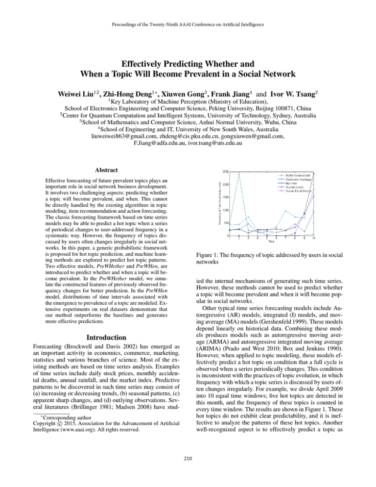
Figure 1: The frequency of topic addressed by users in social
networks
ied the internal mechanisms of generating such time series.
However, these methods cannot be used to predict whether
a topic will become prevalent and when it will become popular in social networks.
Other typical time series forecasting models include Autoregressive (AR) models, integrated (I) models, and moving average (MA) models (Gershenfeld 1999). These models
depend linearly on historical data. Combining these models produces models such as autoregressive moving average (ARMA) and autoregressive integrated moving average
(ARIMA) (Prado and West 2010; Box and Jenkins 1990).
However, when applied to topic modeling, these models effectively predict a hot topic on condition that a full cycle is
observed when a series periodically changes. This condition
is inconsistent with the practices of topic evolution, in which
frequency with which a topic series is discussed by users often changes irregularly. For example, we divide April 2009
into 10 equal time windows; five hot topics are detected in
this month, and the frequency of these topics is counted in
every time window. The results are shown in Figure 1. These
hot topics do not exhibit clear predictability, and it is ineffective to analyze the patterns of these hot topics. Another
well-recognized aspect is to effectively predict a topic as
Introduction
Forecasting (Brockwell and Davis 2002) has emerged as
an important activity in economics, commerce, marketing,
statistics and various branches of science. Most of the existing methods are based on time series analysis. Examples
of time series include daily stock prices, monthly accidental deaths, annual rainfall, and the market index. Predictive
patterns to be discovered in such time series may consist of
(a) increasing or decreasing trends, (b) seasonal patterns, (c)
apparent sharp changes, and (d) outlying observations. Several literatures (Brillinger 1981; Madsen 2008) have stud∗
Corresponding author
c 2015, Association for the Advancement of Artificial
Copyright Intelligence (www.aaai.org). All rights reserved.
210
2011). DTM extends the classic state space models to specify a statistical model of topic evolution and then develops
efficient approximate posterior inference techniques for determining the evolving topics from a sequential collection of
documents.
Forecasting Actions Agarwal, Chen, and Elango (2009)
exploit the Gamma-Poisson model to estimate click-through
rates (number of clicks per display) in the context of content recommendation. Matsubara et al. (2012) introduce the
TriMine method which automatically finds patterns in huge
collections of complex events and forecasts future events.
Tan et al. (2010) propose a Noise Tolerant Time-varying
Factor Graph Model (NTT-FGM) for modeling and predicting social actions. NTT-FGM simultaneously models social
network structure, user attributes and user action history for
better prediction of users’ future actions. Shi et al. (2009)
study the pattern of user participation behaviors, and the feature factors that influence such behaviors on different forum
data sets.
The above methods make use of time series analysis to
predict a personal action such as whether a user will discuss specific topic on his microblogs (tweets), or how many
clicks will be received the next day from a specific user.
They aim to gain more insights into the micro-level for forecasting actions. Our work mainly focuses on finding macrolevel mechanisms for predicting whether and when a topic
will become hot in social networks.
Time Series Pattern Discovery Time series has been
used for similarity search and pattern discovery in series and
sequence data (Matsubara, Sakurai, and Yoshikawa 2009;
Sakurai, Faloutsos, and Yamamuro 2007). For instance, Papadimitriou, Brockwell, and Faloutsos (2004) apply wavelet
transform to capture patterns of time series and introduce
a method of discovering optimal local patterns in Papadimitriou and Yu (2006), which concisely describes the main
trends in a time series. Approaches for regression on time
series and streams include Chen et al. (2002) and Palpanas
et al. (2004). They both estimate the best fit of a given function for forecasting rules in time series.
The above methods address the following problem: Given
a time series which exhibits a clear periodicity, how can a
pattern which concisely describes the main trends in the series be learned. In social networks, the topic frequency series
discussed by users often do not exhibit a clear periodicity. It
is likely that topic frequency series does not form a continuous sequence, rather, it has only a small number of values.
This makes it difficult to use the above methods to predict
hot topic trends, and especially to address the whether and
when problems.
early as possible to capture important events or outcomes,
in particular, to determine whether and when a topic will
become popular. The existing methods (Gershenfeld 1999;
Chen et al. 2002; Palpanas et al. 2004) focus on predicting
the topic frequency based on the observed historical appearance frequency of the topic. These methods face a number
of challenges in practice; for example, they cannot address
the following scenarios: (1) With the three-day frequency of
a topic involved in a social network, will it become a hot
topic in the near future? To address this question, both qualitative and quantitative analysis is necessary. For instance,
many web-sites recommend the Top 10 hot news, movies or
music based on the sum of the click rate over a recent period
of time. However, if the change in click rate is big, or there is
an apparent sharp change in the click rate, an item may suddenly become popular even though the sum of the click rate
is low. Our experimental results show that these methods are
not effective in predicting whether a topic is hot.
Once we can predict whether a topic will become hot in
the near future, another question arises: (2) When will a
topic become hot and interesting to many users (rather than
individuals) in a social network? A quantitative answer to
this question challenges the existing time series-based forecasting models which need intensive human interaction before an answer can be reached, and recommendation methods (Konstan and Riedl 2012; Jannach 2011) which focus
on recommending items for individual users and consistent
changes. Although it appears that we predict when a topic
will become hot based on the observed increased rate of frequency of involvement with this topic by users within a few
days, our experimental results with this method have proved
to be mostly invalid, except for determining that the change
in topic frequency is smooth. This is inconsistent with the
reality in social networks, in which topic frequency changes
stochastically.
This work addresses the above problems of predicting
whether and when a topic will become hot. Motivated by
the assumption that the trend of a topic’s popularity at the
current moment is relevant to the behaviors of the topic in
the previous time period, we propose a generic probabilistic
framework which incorporates the pattern of topic evolution
identified in the previous time period into the prediction of
its dynamics at the current time. Two effective probabilistic
models are then built to address the above questions, i.e. predicting whether and when a topic will become hot. Specifically, the PreWHether model is proposed to simulate the
extracted features of previously observed topic dynamics,
which determine whether it will become hot. The PreWHen
model further models the distributions of time intervals from
the emergence of the topic to its prevalence by using the
Gamma distribution, which can identify when a topic becomes popular.
Problem Statement
In this section, we formalize the problem of forecasting
whether and when a topic will become hot in a social network in the near future. We divide a month into T time windows and the length of every time window is t hours. Given
a topic which first emerges at the i-th time window, and its
frequency of appearing in the network at i-th,· · · ,i + m-th
time windows, if the topic is not prevalent at i + m-th time
window, the task here is to forecast whether it will become
Related Work
Evolution of Topics A number of methods have been proposed for analyzing the temporal evolution of topics in document collections, such as the dynamic topic model (DTM)
(Blei and Lafferty 2006), topics over time (TOT) (Xuerui
and Andrew 2006), trend analysis model (TAM) (Kawamae
211
Proposed Models
hot and at which future time window. We formalize the problem as follows.
Let K be a set of topics, K = {ki |ki is the set of
keywords}. xki ,j denotes the frequency of topic ki involved
at the j-th time window. We define a hot topic as follows:
Definition 1. (Hot Topic) Let S =
m
P
The PreWHether Model
Here we specify and present an effective model,
PreWHether, for predicting whether a topic will become hot. Let C1 denote a hot topic, and C0 represent a
topic that is not hot. Given topic ki and the feature vector
X, a more powerful approach to forecasting Problem 1 is to
model the posterior probability distributions p(C0 |X) and
p(C1 |X). These two distributions are then used to make an
optimal decision.
Based on Bayes’ theorem, the posterior probability
p(C1 |X) can be written as
xki ,j , 0 ≤ m ≤ T .
j=0
If S ≥ α (where α is the threshold), then topic ki is a hot
topic.
Assume users in the network first talk about topic ki at the
j-th time window. We get the time series data, {xki ,j , · · · ,
m
P
xki ,t < α, we aim to forecast
xki ,m }, j < m < T . If
p(C1 |X) =
t=j
whether topic ki will become a hot topic at a later time window based on features of the time series data. We use vector
X = (x1ki , · · · , xnki ) to denote the features of the observed
time series data. For example, we can use the sum, growth
rate, mean and variance and so on as the features of the time
series data. Accordingly, we state Problem 1 as follows.
p(C1 )p(X|C1 )
p(C1 )p(X|C1 ) + p(C0 )p(X|C0 )
(1)
If the likelihood and prior probability distributions in Eq.(1)
are obtained, we can determine Problem 1. Below, we discuss how to model the likelihood and prior probability distributions in Eq.(1).
The dimension of feature vector X of topic ki is 3: sum
denoted as x1ki , average rate of change denoted as x2ki , standard deviation denoted as x3ki . Assume x1ki , x2ki , x3ki are mutual conditionally independent given C1 or C0 . The likelihood probability p(X|C1 ) can be written as
Problem 1. (Whether a Topic Hot) We observe the time sem
P
ries data {xki ,j , · · · , xki ,m }, j < m < T . If
xki ,t < α,
t=j
p(X|C1 ) = p(x1ki |C1 )· p(x2ki |C1 ) · p(x3ki |C1 )
we aim to forecast whether topic ki will be hot at a later
time window based on X which is the feature vector of the
time series data. That is, whether ∃, m < ≤ T, to satisfy
P
xki ,t ≥ α.
(2)
We analyze the features of sum, average rate of change,
standard deviation and model likelihood probability distributions for these three dimension variables respectively.
By observing the data characteristics of topic evolution,
we find that the probability of topic ki which belongs to C1
is proportional to x1ki . If the propagation sources of topic
ki are influential on the whole network, there will be more
people talking about this topic, and x1ki will become bigger.
If the topic is interesting to people, more people will focus
on this topic at the initial time windows, so we obtain much
bigger x1ki . We suppose there are two factors controlling x1ki :
one is related to the propagation sources of the topic, while
the other is related to the attraction of the topic to people.
Suppose x1ki is a continuous variable, we use the Beta distribution to model the likelihood of probability distributions.
The shape of the probability density function of the Beta distribution changes with different parameter settings. We can
use the increasing function to model p(x1ki |C1 ) and the decreasing function to model p(x1ki |C0 ). The different parameters denote different classes.
We observe that x2ki tends to have concentrated distribution at different intervals for different classes. Assume that
x2ki is a continuous variable. Considering that x2ki varies
from negative infinity to positive infinity, we can use Gaussian distribution to model p(x2ki |C1 ) and p(x1ki |C0 ).
We also observe that x3ki tends to have concentrated distribution at different intervals for different classes. Assume
that x3ki is a continuous variable. Since x3ki is nonnegative,
and we need an unimodal distribution to characterize it, the
Gamma distribution is frequently used to model p(x3ki |C1 )
and p(x3ki |C0 ).
t=j
If a topic is predicted to be a hot one, we aim to forecast
when it becomes hot. This leads to Problem 2.
Problem 2. (When a Topic Will Become Hot) Given a hot
topic ki which emerges at j-th time window, we aim to find
η
P
η-th (j ≤ η ≤ T ) time window, satisfying
xki ,t ≥ α.
t=j
In our experiments, we divide a month into 90 time windows and the length of every time window is 8 hours (T =
90, t = 8). For every topic, we set a fixed length of observed time series data. Suppose users in the network first
talk about topic ki at the j-th time window, then let us
observe the evolution of the topic within 9 time windows
{xki ,j , · · · , xki ,j+8 } (namely three days). In our framework, we consider the choice of 3 features that are usually used in statistics and practice(i.e. sum, average rate of
change and standard deviation), to measure the topic evolution, so the feature vector X is denoted as: X = (sum,
average rate of change, standard deviation), where sum=
j+8
j+7
P
P xki ,t+1 −xki ,t
xki ,t , average rate of change= 81 ·
, stanxki ,t
t=j
t=j
s
j+8
P
dard deviation= 19 ·
(xki ,t − µ̂)2 where µ̂ is the mean
t=j
of {xki ,j , · · · , xki ,j+8 }.
212
Theorem 1. (Log-convex for beta function) Let x > 0, y >
0, the Beta function can be written as
Z 1
B(x, y) =
ux−1 · (1 − u)y−1 du
(8)
To keep the notation clean, we denote topic ki by i.
Suppose we have a data set D = (x1i , x2i , x3i , ti ) where
i = 1, · · · , n. Here ti = 1 denotes class C1 and ti = 0 denotes class C0 . Let the prior class probability be p(C1 ) = β,
so that p(C0 ) = 1 − β. a, b, µ, σ, c, d are the parameters
which describe each distribution. i.e. µ, σ stand for the mean
and variance of Gaussian distribution; a, b and c, d represent
the shape and scale parameters of Beta and Gamma distribution respectively. For a feature vector X = {x1i , x2i , x3i }
from class C1 , we have ti = 1 and hence
0
Then B(x, y) is a log-convex function of x and y.
Assume that fi , 1 ≤ i ≤ n are convex functions, and
wi ≥ 0, 1 ≤ i ≤ n
n
X
f=
wi · fi
(9)
i=1
p(X, C1 ) = p(C1 )p(X|C1 )
Then Eq.(9)) is a convex function.
Based on Theorem 1 and Eq.(9)), we have the following
theorem:
Theorem 2. (Convexity for Eq.(7)) The optimization problem of maximizing the log of the Beta distribution function
represented by Eq.(7) is a convex optimization problem.
Let
L(x2i , x3i ; µ1 , σ1 , µ0 , σ0 , c1 , d1 , c0 , d0 )
=
n
Q
2
ti
2
1−ti
N (xi |µ1 , σ1 )
·
N (xi |µ0 , σ0 )
·
=β · Beta(x1i |a1 , b1 ) · N (x2i |µ1 , σ1 ) · Gamma(x3i |c1 , d1 )
(3)
Similarly for class C0 , we have ti = 0 and hence
p(X, C0 ) = p(C0 )p(X|C0 )
=(1 − β) · Beta(x1i |a0 , b0 ) · N (x2i |µ0 , σ0 )
·
(4)
i=1
Gamma(x3i |c0 , d0 )
Gamma(x3i |c1 , d1 )ti · Gamma(x3i |c0 , d0 )1−ti . To estimate
the parameters of Gaussian and Gamma distributions, we
solve the problem
min − ln L(x2i , x3i ; µ1 , σ1 , µ0 , σ0 , c1 , d1 , c0 , d0 )
(10)
s.t.
σ1 > 0, σ0 > 0
c1 > 0, d1 > 0, c0 > 0, d0 > 0
We can get a local optimal solution of Eq.(10).
To keep the notation clean, we write ω1
=
(a1 , b1 , µ1 , σ1 , c1 , d1 ) and ω0 = (a0 , b0 , µ0 , σ0 , c0 , d0 ).
Thus the likelihood function is given by
p(D|β, ω1 , ω0 )
n
Y
= [β · Beta(x1i |a1 , b1 ) · N (x2i |µ1 , σ1 )
i=1
·
·
(5)
The PreWHen Model
Gamma(x3i |c1 , d1 )]ti · [(1 − β) · Beta(x1i |a0 , b0 )
N (x2i |µ0 , σ0 ) · Gamma(x3i |c0 , d0 )]1−ti
We describe an effective model, PreWHen, for predicting
when a topic will become a hot topic. We observe the time
series of hot topics in the data set. Most of the topics tend
to become hot at a constant time window from their first
emergence in the network. Assume topic ki emerges at the
j-th time window, and it becomes hot at η-th (j ≤ η ≤ T )
η
P
time window which means that
xki ,t ≥ α. Let x denote
β, ω1 , ω0 can be obtained by solving the problem
max ln p(D|β, ω1 , ω0 )
s.t. a1 > 0, b1 > 0, a0 > 0, b0 > 0
σ1 > 0, σ0 > 0, 0 ≤ β ≤ 1
c1 > 0, d1 > 0, c0 > 0, d0 > 0
(6)
t=j
the difference between xki ,η and xki ,j for all the hot topic,
x = xki ,η − xki ,j . Assume x is continuous variable. Since
x is nonnegative, we use unimodal Gamma distribution to
characterize it. Let ∆x be a small interval of x. We set the
length of ∆x to 1.
Estimation of parameters. Because the likelihood probability p(X|C1 ) and p(X|C0 ) are the product of three factors and the parameters of Beta distribution, Gaussian distribution and Gamma distribution are mutually independent
in Eq.(6). We estimate the respective parameters of the three
distributions accordingly.
n
Q
Let L(x1i ; β, a1 , b1 , a0 , b0 ) =
(β · Beta(x1i |a1 , b1 ))ti ·
p(x) ∼
(11)
= Gamma(x|ϕ, χ) · ∆x
We need to estimate the parameters in Eq.(11). The
maximum likelihood estimation of the Gamma distribution
function is used to estimate ϕ and χ. Let L(xi ; ϕ, χ) =
n
Q
Gamma(xi |ϕ, χ). Given observations x1 , · · · , xn , the
i=1
[(1−β)·Beta(x1i |a0 , b0 )]1−ti . For estimating the parameters
of the Beta distribution, we need to solve the problem below:
i=1
min − ln L(x1i ; β, a1 , b1 , a0 , b0 )
s.t. a1 > 0, b1 > 0, a0 > 0, b0 > 0
0≤β≤1
problem is
min − ln L(xi ; ϕ, χ)
(12)
s.t.
ϕ > 0, χ > 0
Eq.(12) is not a convex optimization problem, so we adopt a
local optimal solution.
A topic will be a hot one at the interval of the Gamma
distribution mode in the maximum probability.
(7)
The solution to Eq.(7) is unique, computable and consistent.
Based on Hölder’s inequality (Hewitt and Stromberg
1965), we have the following two theorems:
213
Table 1: The mean of Precision, Recall and F1-Measure with
hot topic threshold α = 800
3→1
4→1
5→1
6→1
7→1
Figure 2: The percentage of hot topics with different hot
topic thresholds α
We develop the PreWHether and PreWHen models to discover hot topic patterns based on the previous time series data of hot topics. Given a new topic knew and its
corresponding time series data {xki ,j , · · · , xki ,m }, we can
predict whether the topic is hot based on the learned hot
topic patterns. Firstly, we calculate the feature vector of
topic knew , X = (x1knew , x2knew , x3knew ); We then compute
p(C1 |X) and p(C0 |X) based on the learned parameters.
Lastly, we calculate p(C1 |X) with p(C0 |X). If p(C1 |X) is
bigger than p(C0 |X), we predict it as a hot topic; otherwise,
it is not a hot topic. Assuming that topic knew is a hot one,
we predict it will become hot at the interval of the Gamma
distribution mode in the maximum probability based on the
learned PreWHen model.
Experimental Evaluation
Data Sets
The data sets are from Meme Tracker1 (Leskovec, Backstrom, and Kleinberg 2009). They consist of a set of
(P, T i, Q), P is the URL which denotes users, T i is the
time point, Q is the text that a user P typed at time point
T i. We extract the data from August 2008 to April 2009.
Every month is divided into 90 time windows and the length
of every time window is 8 hours.
We extract the news topic from a website 2 , and keywords
reflecting different topics are extracted. If text Q involves
keywords that reflect a specific topic ki by user P , we consider that P talks about ki at the corresponding time point
T i. For every month, we extract 15 news topics and corresponding keywords for every topic. We count the frequency
of every topic that is involved by users for 90 time windows
and observe whether these topics are hot. The total number
of topics extracted is 120.
Performance Evaluation for PreWHether
The percentage of hot topics for different hot topic thresholds is shown in Figure 2. We see the percentage of hot topics decrease with the increase of the hot topic threshold α.
Assuming the percentage of hot topics is between 20% and
50%, we select 800, 1100 and 1400 as the values of the hot
topic threshold α.
2
M-Recall
0.7026
0.7831
0.8958
0.9444
0.9167
M-F1-Measure
0.6176
0.6971
0.7680
0.7746
0.7503
Baseline Methods. The existing algorithms in recommendation systems, topic modeling, and time series can be
used to handle the whether and when problems discussed in
this paper. As our proposed approach is based on time series
analysis, we compare our method with the following methods of predicting whether a topic will become hot:
Naive: Recommended the top 20 per cent of topics to
users as hot topics based on the sum of frequency observed
in 9 time windows of topics which have user involvement
from the emergence of these topics.
Ar: Autoregressive (AR(4)) model is used to predict the
topic frequency of the 10-th time window from its emergence. The top 20 percent topics are regarded as hot based
on the values pedicted by the AR(4) model. We used the
same three features for the PreWHether model to train the
AR model.
Regre-3: Polynomial regression model with degree 3 is
used to model the topic frequency of the observed 9 time
windows from emergence. In this model, a topic is judged
to be hot or not in a step by step process until the answer is
obtained.
Evaluation Metrics. We evaluate the proposed method in
terms of Precision, Recall and F1-Measure, and compare it
with the baseline methods to validate the effectiveness of the
proposed method.
We have 9 months’ topics in total. Let α = 800. Topics of 7 months are treated as the training set to predict
the next month’s topics. First, we use the data set of the
first to the seventh month as the training set to predict the
eighth month’s topics and compute Precision, Recall, and
F1-Measure. Then the data set of the second to eighth month
is used as the training set to predict the ninth month’s topics and compute Precision, Recall, and F1-Measure. Last,
we separately calculate the mean of Precision, Recall, and
F1-Measure. In our experiment, the topic data of 3 months,
4 months, 5 months and 6 months respectively is used as a
training set to predict the corresponding next month’s topics, and we obtain similar results. The experiment results
are shown in Table 1, and M-Precision, M-Recall and MF1-Measure denote the mean of Precision, Recall, and F1Measure respectively. 7→1 means that the topic data of 7
months is used as a training set to predict the next month’s
topics. The meanings of 3→1, 4→1, 5→1 and 6→1 are
similar to the 7→1. Table 1 shows that the M-F1-Measure
increases and the M-F1-Measure of 5→1 almost equals to
that of 6→1 and 7→1. We therefore execute the next experiment under the condition of 5→1. Let α = 800, we
use the PreWHether model to predict the sixth, seventh,
Hot Topic Prediction
1
M-Precision
0.5510
0.6282
0.6722
0.6566
0.6350
http://snap.stanford.edu/data/memetracker9.html
http://www.infoplease.com
214
Figure 4: The performance evaluation for PreWHen against
baseline methods
Figure 3: The performance evaluation for PreWHether and
baseline methods
come hot by our method and the Naive method, the deviation
between the predicted value and true value is then obtained.
We forecast all hot topics of one month, and use the Mean
and Standard Deviation of these deviations to evaluate the
performance of PreWHen against the Naive method.
Certain models require step by step judgement until the
time window for a hot topic is achieved. Therefore, we do
not use these models to tackle Problem 2.
Let α = 800, we use PreWHen and the Naive method respectively to predict when topics of the sixth month become
hot, and compute the corresponding Mean and Standard Deviation, likewise for the seventh, eighth and ninth months.
Both methods are separately tested based on patterns of the
previous five months of hot topics and the rise rate of the observed frequency in 9 time windows of each hot topic. The
experiments of α = 1100, 1400 are similar to α = 800. Figure 4 shows the prediction performance of two approaches
on three different hot topic thresholds α.
Performance Comparison. Our method PreWHen consistently achieves better performance. In terms of Mean, the
average deviation of our method is smaller than the baseline method by fifty. In terms of Standard Deviation, our approach fluctuates a little, while the Naive method fluctuates
much more than ours. The baseline method works well in
predicting hot topics of the eighth month. This is because
the average rise rate of frequency of these hot topics tends
to be smooth, whereas such a case seldom appears. The proposed method provides effective answers for Problem 2.
eighth and ninth month topics based on the previous five
months of topic data and compute the corresponding Precision, Recall, and F1-Measure for each predicted month.
Baseline methods are also used to predict the sixth, seventh,
eighth and ninth month topics and we obtain the corresponding Precision, Recall and F1-Measure. The experiments of
α = 1100, 1400 are similar to α = 800. Figure 3 shows
the prediction performance of different approaches based on
the three different hot topic thresholds α with the following
observations. Due to the page limitation, we only report the
performance of F1-Measure here in Figure 3. The month in
the x-axis of Figure 3 is the ground-truth month value.
Performance Comparison. We can see that our model
PreWHether consistently achieves better performance than
the baseline methods. In terms of F1-Measure, PreWHether
achieves more than +60% with α = 800, 1100. Even though
the number of hot topics in the training dataset is fewer when
α = 1400, our method still mostly achieves an F1-Measure
of +40%. Given the experiments shown in Figure 3, not all
baselines do not work better than the proposed method in all
cases. The Naive and Ar methods depend on only one metric
of the past few frequency values of a single series to address
Problem 1. The series of hot topic frequency discussed by
users does not change periodically through time and the observed data is very limited. As a result, these methods cannot
achieve a better prediction for Problem 1. Regre-3 may have
a good fit to a set of past data, but it is not the most useful
model for predicting future values. Fitting past values and
forecasting future values are two quite different things. The
regression models do not work well for solving Problem 1.
The hot topic trends of one month are related to hot topic
patterns of several previous months, and our approach incorporates the information of hot topic patterns of several
previous months to mine more effective hot topic patterns.
In summary, our model effectively makes better predictions
than the baseline approaches.
Conclusions
In this paper, we discuss two practical but challenging issues, i.e., forecasting whether and when a topic will become
a hot topic in a social network. Limited existing research
can be directly applied to address these problems, due to the
uncertainty and restricted information from the related data
characteristics and the involvement of the community in a
network. In this paper, a generic probabilistic framework has
been presented to discover a hot topic evolution pattern for
the effective prediction of the topic prevalence. Two effective probabilistic models, PreWHether and PreWHen, have
been learned to solve the proposed problems. Substantial experiments on real datasets show that our method outperforms
the baselines and makes much better predictions.
Performance Evaluation for PreWHen
Evaluation Metrics. Given a hot monthly topic, we separately forecast the time window in which this topic will be-
215
Acknowledgments
Prado, R., and West, M. 2010. Time Series: Modelling,
Computation and Inference. London: CRC Press.
Sakurai, Y.; Faloutsos, C.; and Yamamuro, M. 2007. Stream
monitoring under the time warping distance. In ICDE,
1046–1055.
Shi, X.; Zhu, J.; Cai, R.; and Zhang, L. 2009. User grouping
behavior in online forums. In KDD, 777–786.
Tan, C.; Tang, J.; Sun, J.; Lin, Q.; and Wang, F. 2010. Social
action tracking via noise tolerant time-varying factor graphs.
In KDD, 1049–1058.
Xuerui, W., and Andrew, M. 2006. Topics over time: A nonmarkov continuous-time model of topical trends. In KDD,
424–433.
This research was supported by the Project 61170091 supported by National Natural Science Foundation of China
and the Australian Research Council Future Fellowship
FT130100746.
References
Agarwal, D.; Chen, B.-C.; and Elango, P. 2009. Spatiotemporal models for estimating click-through rate. In WWW,
21–30.
Blei, D. M., and Lafferty, J. D. 2006. Dynamic topic models.
In ICML, 113–120.
Box, G. E. P., and Jenkins, G. 1990. Time Series Analysis,
Forecasting and Control. San Francisco, CA: Holden-Day,
Incorporated.
Brillinger, D. R. 1981. Time series : data analysis and theory. San Francisco, CA: Holden-Day.
Brockwell, P., and Davis, R. 2002. Introduction to Time
Series and Forecasting. New York: Springer.
Chen, Y.; Dong, G.; Han, J.; Wah, B. W.; and Wang, J.
2002. Multi-dimensional regression analysis of time-series
data streams. In VLDB, 323–334.
Gershenfeld, N. A. 1999. The Nature of Mathematical Modeling. Cambridge: Cambridge University Press.
Hewitt, E., and Stromberg, K. 1965. Real and abstract analysis. A modern treatment of the theory of functions of a real
variable. New York: Springer-Verlag.
Jannach, D. 2011. Recommender systems : an introduction.
New York: Cambridge University Press.
Kawamae, N. 2011. Trend analysis model: trend consists
of temporal words, topics, and timestamps. In WSDM, 317–
326.
Konstan, J. A., and Riedl, J. 2012. Recommender systems: from algorithms to user experience. User Modeling
and User-Adapted Interaction 22:101–123.
Leskovec, J.; Backstrom, L.; and Kleinberg, J. M. 2009.
Meme-tracking and the dynamics of the news cycle. In
KDD, 497–506.
Madsen, H. 2008. Time Series Analysis. London: CRC
Press.
Matsubara, Y.; Sakurai, Y.; Faloutsos, C.; Iwata, T.; and
Yoshikawa, M. 2012. Fast mining and forecasting of complex time-stamped events. In KDD, 271–279.
Matsubara, Y.; Sakurai, Y.; and Yoshikawa, M. 2009. Scalable algorithms for distribution search. In ICDM, 347–356.
Palpanas, T.; Vlachos, M.; Keogh, E. J.; Gunopulos, D.; and
Truppel, W. 2004. Online amnesic approximation of streaming time series. In ICDE, 339–349.
Papadimitriou, S., and Yu, P. S. 2006. Optimal multi-scale
patterns in time series streams. In SIGMOD, 647–658.
Papadimitriou, S.; Brockwell, A.; and Faloutsos, C. 2004.
Adaptive, unsupervised stream mining. VLDB J. 13(3):222–
239.
216