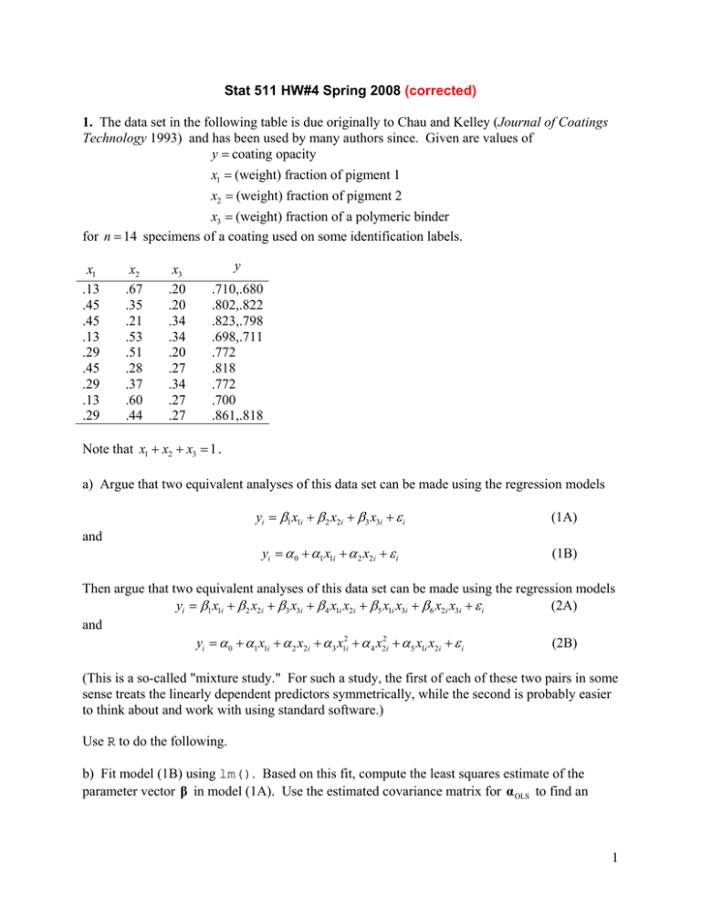
Stat 511 HW#4 Spring 2008 (corrected)
1. The data set in the following table is due originally to Chau and Kelley (Journal of Coatings
Technology 1993) and has been used by many authors since. Given are values of
y = coating opacity
x1 = (weight) fraction of pigment 1
x2 = (weight) fraction of pigment 2
x3 = (weight) fraction of a polymeric binder
for n = 14 specimens of a coating used on some identification labels.
x1
.13
.45
.45
.13
.29
.45
.29
.13
.29
x2
.67
.35
.21
.53
.51
.28
.37
.60
.44
x3
.20
.20
.34
.34
.20
.27
.34
.27
.27
y
.710,.680
.802,.822
.823,.798
.698,.711
.772
.818
.772
.700
.861,.818
Note that x1 + x2 + x3 = 1 .
a) Argue that two equivalent analyses of this data set can be made using the regression models
and
yi = β1 x1i + β 2 x2i + β 3 x3i + ε i
(1A)
yi = α 0 + α1 x1i + α 2 x2i + ε i
(1B)
Then argue that two equivalent analyses of this data set can be made using the regression models
yi = β1 x1i + β 2 x2i + β 3 x3i + β 4 x1i x2i + β 5 x1i x3i + β 6 x2i x3i + ε i
(2A)
and
yi = α 0 + α1 x1i + α 2 x2i + α 3 x12i + α 4 x22i + α 5 x1i x2i + ε i
(2B)
(This is a so-called "mixture study." For such a study, the first of each of these two pairs in some
sense treats the linearly dependent predictors symmetrically, while the second is probably easier
to think about and work with using standard software.)
Use R to do the following.
b) Fit model (1B) using lm(). Based on this fit, compute the least squares estimate of the
parameter vector β in model (1A). Use the estimated covariance matrix for α OLS to find an
1
estimated covariance matrix for β OLS . Then fit model (1A) directly using lm(). (A " −1 " in the
model specification will fit a no-intercept regression.)
c) Fit model (2B) to these data and normal plot standardized residuals.
d) In the model (2B) test H 0 : α 3 = α 4 = α 5 = 0 . Report a p-value. Does quadratic curvature in
response (as a function of the x 's) appear to be statistically detectable?
e) Use some multivariate calculus on the fitted quadratic equation and find the location
( x1 , x2 ) of an absolute maximum. Use R matrix calculations to find 90% two-sided confidence
limits for the mean response here. Then find 90% two-sided prediction limits for a new response
from this set of conditions.
2. (Testing “Lack of Fit” … See Section 6.6 of Christensen) Suppose that in the usual linear
model
Y = Xβ + ε
X is of full rank ( k ). Suppose further that there are m < n distinct rows in X and that m > k .
One can then make up a "cell means" model for Y (where observations having the same
corresponding row in X are given the same mean response) say
Y = X *μ + ε
This model puts no restrictions on the means of the observations except that those with identical
corresponding rows of X are equal. It is the case that C ( X ) ⊂ C ( X * ) and it thus makes sense to
test the hypothesis H 0 :EY ∈ C ( X ) in the cell means model. This can be done using
F=
Y ' ( PX* − PX ) Y / ( m − k )
Y ' ( I − PX* ) Y / ( n − m )
and this is usually known as testing for "lack of fit."
Use R and matrix calculations to find a p-value for testing lack of fit to the quadratic regression
model (2B) in Problem 1.
3. Below is a small table of fake 2-way factorial data. Enter them into R in three vectors of
length n = 12 . Call these vectors "y", "A", and "B".
Level 1 of A
Level 2 of A
Level 3 of A
Level 1 of B
12
8
10
Level 2 of B
13,14,15
10
13
Level 3 of B
20
6,7
7
a) Create and print out an R data frame using the commands
> d<-data.frame(y,A,B)
> d
2
b) Turn the numerical variables A and B into variables that R will recognize as levels of
qualitative factors by issuing the commands
> d$A<-as.factor(d$A)
> d$B<-as.factor(d$B)
Then compute and print out the cell means by typing
> means<-tapply(d$y,list(d$A,d$B),mean)
> means
You may find out more about the function tapply by typing
> ?tapply
c) Make a crude interaction plot by doing the following. First type
> x.axis<-unique(d$B)
to set up horizontal plotting positions for the sample means. Then make a "matrix plot" with
lines connecting points by issuing the commands
> matplot(c(1,3),c(5,25),type="n",xlab="B",ylab="Mean
Response",main="y")
> matlines(x.axis,means,type="b")
The first of these commands sets up the axes and makes a dummy plot with invisible points
"plotted" at (1,5) and (3, 25) . The second puts the lines and identifying A levels (as plotting
symbols) on the plot.
d) Set the default for the restriction used to create a full rank model matrix, run the linear models
routine and find both sets of "Type I" sums of squares by issuing the following commands
>
>
>
>
>
options(contrasts=c("contr.sum","contr.sum"))
lm.out1<-lm(y~A*B,data=d)
summary.aov(lm.out1,ssType=1)
lm.out2<-lm(y~B*A,data=d)
summary.aov(lm.out2,ssType=1)
See if anything changes if you ask R to compute "Type III" sums of squares by issuing the
command
> summary.aov(lm.out1,ssType=3)
(In the past R has failed to respond to the request for Type III sums of squares without warning
you that it is going to fail to do so.)
3
e) Start over with this problem, doing the calculations "from scratch" using your basic linear
models knowledge and matrix calculations in R. Compute all of Type I, Type II and Type III
sums of squares here, using the sum restriction in the first two cases (and the order of factors
A,B). Then compute Type I and Type II sums of squares using the SAS baseline restriction.
f) Now suppose that by some misfortune, the observation from the (1,3) cell of this complete
3 × 3 factorial somehow gets lost and one has only n = 11 observations from k = 8 cells (and thus
"incomplete factorial" data). Test the hypothesis that at least for the cells where one has data,
((
there are no interactions, i.e. E Y ∈ C 1 | Xα * | X β *
)) . (Note that this matrix (1 | X
α*
)
| X β * should
be of full rank.)
g) In the incomplete factorial context of part f), the function μ + α1* + β3* is estimable. What is
the OLS estimate for it? (Note that this is the mean response for the missing cell only if the same
no-interaction model used to describe the 8 cells extends to the 9th. This is the kind of
assumption one makes in regression analysis when using a fitted prediction equation to estimate
a mean response at a set of conditions not in one's original data set. It might well be argued,
however, that the link between observed and unobserved conditions is intuitively stronger with
quantitative factors than with qualitative factors.)
4