Proceedings of the Thirtieth AAAI Conference on Artificial Intelligence (AAAI-16)
SentiCap: Generating Image Descriptions with Sentiments
Alexander Mathews∗ , Lexing Xie∗† , Xuming He†∗
∗
The Australian National University, † NICTA
alex.mathews@anu.edu.au, lexing.xie@anu.edu.au, xuming.he@nicta.com.au
Abstract
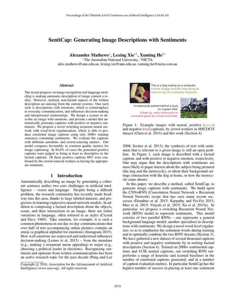
This is a dog resting on a computer.
A white shaggy beautiful dog laying its
head on top of a computer keyboard.
The recent progress on image recognition and language modeling is making automatic description of image content a reality. However, stylized, non-factual aspects of the written
description are missing from the current systems. One such
style is descriptions with emotions, which is commonplace
in everyday communication, and influences decision-making
and interpersonal relationships. We design a system to describe an image with emotions, and present a model that automatically generates captions with positive or negative sentiments. We propose a novel switching recurrent neural network with word-level regularization, which is able to produce emotional image captions using only 2000+ training
sentences containing sentiments. We evaluate the captions
with different automatic and crowd-sourcing metrics. Our
model compares favourably in common quality metrics for
image captioning. In 84.6% of cases the generated positive
captions were judged as being at least as descriptive as the
factual captions. Of these positive captions 88% were confirmed by the crowd-sourced workers as having the appropriate sentiment.
1
A motorcycle parked behind a truck
on a green field.
A beat up, rusty motorcycle on
unmowed grass by a truck and trailer.
Figure 1: Example images with neural, positive (green)
and negative (red) captions, by crowd workers in MSCOCO
dataset (Chen et al. 2015) and this work (Section 4).
2008; Socher et al. 2013), the synthesis of text with sentiment that is relevant to a given image is still an open problem. In Figure 1, each image is described with a factual
caption, and with positive or negative emotion, respectively.
One may argue that the descriptions with sentiments are
more likely to pique interest about the subject being pictured
(the dog and the motocycle), or about their background settings (interaction with the dog at home, or how the motocycle came about).
In this paper, we describe a method, called SentiCap, to
generate image captions with sentiments. We build upon
the CNN+RNN (Convolution Neural Network + Recurrent
Neural Network) recipe that has seen many recent successes (Donahue et al. 2015; Karpathy and Fei-Fei 2015;
Mao et al. 2015; Vinyals et al. 2015; Xu et al. 2015a). In
particular, we propose a switching Recurrent Neural Network (RNN) model to represent sentiments. This model
consists of two parallel RNNs – one represents a general
background language model; another specialises in descriptions with sentiments. We design a novel word-level regularizer, so as to emphasize the sentiment words during training
and to optimally combine the two RNN streams (Section 3).
We have gathered a new dataset of several thousand captions
with positive and negative sentiments by re-writing factual
descriptions (Section 4). Trained on 2000+ sentimental captions and 413K neutral captions, our switching RNN outperforms a range of heuristic and learned baselines in the
number of emotional captions generated, and in a number
of caption evaluation metrics. In particular SentiCap has the
highest number of success in placing at least one sentiment
Introduction
Automatically describing an image by generating a coherent sentence unifies two core challenges in artificial intelligence – vision and language. Despite being a difficult
problem, the research community has recently made headway into this area, thanks to large labeled datasets, and progresses in learning expressive neural network models. In addition to composing a factual description about the objects,
scene, and their interactions in an image, there are richer
variations in language, often referred to as styles (Crystal
and Davy 1969). Take emotion, for example, it is such a
common phenomena in our day-to-day communications that
over half of text accompanying online pictures contains an
emoji (a graphical alphabet for emotions) (Instagram 2015).
How well emotions are expressed and understood influences
decision-making (Lerner et al. 2015) – from the mundane
(e.g., making a restaurant menu appealing) to major (e.g.,
choosing a political leader in elections). Recognizing sentiment and opinions from written communications has been
an active research topic for the past decade (Pang and Lee
c 2016, Association for the Advancement of Artificial
Copyright Intelligence (www.aaai.org). All rights reserved.
3574
tive area of research (Pang and Lee 2008; Socher et al.
2013). Several teams (Nakagawa, Inui, and Kurohashi 2010;
Täckström and McDonald 2011) designed sentence models
with latent variables representing the sentiment. Our work
focuses on generating sentences and not explicitly modelling
sentiment using hidden variables.
word into the caption, 88% positive (or 72% negative) captions are perceived by crowd workers as more positive (or
negative) than the factual caption, with a similar descriptiveness rating.
2
Related Work
Recent advances in visual recognition have made “an image
is a thousand words” much closer to reality, largely due to
the advances in Convolutional Neural Networks (CNN) (Simonyan and Zisserman 2015; Szegedy et al. 2015). A
related topic also advancing rapidly is image captioning,
where most early systems were based on similarity retrieval
using objects and attributes (Farhadi et al. 2010; Kulkarni et al. 2011; Hodosh, Young, and Hockenmaier 2013;
Gupta, Verma, and Jawahar 2012), and assembling sentence
fragments such as object-action-scene (Farhadi et al. 2010),
subject-verb-object (Rohrbach et al. 2013), object-attributeprepositions (Kulkarni et al. 2011) or global image properties such as scene and lighting (Nwogu, Zhou, and Brown
2011). Recent systems model richer language structure,
such as formulating a integer linear program to map visual
elements to the parse tree of a sentence (Kuznetsova et al.
2014), or embedding (Xu et al. 2015b) video and compositional semantics into a joint space.
Word-level language models such as RNNs (Mikolov
et al. 2011; Sutskever, Martens, and Hinton 2011) and
maximum-entropy (max-ent) language models (Mikolov et
al. 2011) have improved with the aid of significantly larger
datasets and more computing power. Several research teams
independently proposed image captioning systems that combine CNN-based image representation and such language
models. Fang et al. (2015) used a cascade of word detectors from images and a max-ent model. The Show
and Tell (Vinyals et al. 2015) system used an RNN as the
language model, seeded by CNN image features. Xu et
al. (2015a) estimated spatial attention as a latent variable,
to make the Show and Tell system aware of local image information. Karpathy and Li (2015) used an RNN to generate a sentence from the alignment between objects and
words. Other work has employed multi-layer RNNs (Chen
and Zitnick 2015; Donahue et al. 2015) for image captioning. Most RNN-based multimodal language models use the
Long Short Term Memory (LSTM) unit that preserves longterm information and prevents overfitting (Hochreiter and
Schmidhuber 1997). We adopt one of the competitive systems (Vinyals et al. 2015) – CNN+RNN with LSTM units
as our basic multimodal sentence generation engine, due to
its simplicity and computational efficiency.
Researchers have modeled how an image is presented,
and what kind of response it is likely to elicit from viewers, such as analyzing the aesthetics and emotion in images (Murray, Marchesotti, and Perronnin 2012; Joshi et al.
2011). More recently, the Visual SentiBank (Borth et al.
2013) system constructed a catalogue of Adjective-NounPairs (ANPs) that are frequently used to describe online images. We build upon Visual SentiBank to construct sentiment vocabulary, but to the best of our knowledge, no existing work tries to compose image descriptions with desired sentiments. Identifying sentiment in text is an ac-
3
Describing an Image with Sentiments
Given an image I and its Dx -dimensional visual feature
x ∈ RDx , our goal is to generate a sequence of words
(i.e. a caption) Y = {y1 , · · · , yT } to describe the image
with a specific style, such as expressing sentiment. Here
yt ∈ {0, 1}V is 1-of-V encoded indicator vector for the tth
word; V is the size of the vocabulary; and T is the length of
the caption.
We assume the sentence generation involves two underlying mechanisms, one of which focuses on the factual description of the image while the other describes the image
content with sentiments. We formulate such caption generation process using a switching multi-modal language model,
which sequentially generates words in a sentence. Formally,
we introduce a binary sentiment variable st ∈ {0, 1} for every word yt to indicate which mechanism is used. At each
time step t, our model produces the probability of yt and the
current sentiment variable st given the image feature x and
the previous words y1:t−1 , denoted by p(yt , st |x, y1:t−1 ).
We generate the word probability by marginalizing over the
sentiment variable st :
p(yt |x, y1:t−1 ) =
p(yt |st , x, y1:t−1 )p(st |x, y1:t−1 ) (1)
st
Here p(yt |st , ·) is the caption model conditioned on the sentiment variable and p(st |·) is the probability of the word sentiment. The rest of this section will introduce these components and model learning in detail.
3.1
Switching RNNs for Sentiment Captions
We adopt a joint CNN+RNN architecture (Vinyals et al.
2015) in the conditional caption model. Our full model combines two CNN+RNNs running in parallel: one capturing
the factual word generation (referred to as the background
language model), the other specializing in words with sentiment. The full model is a switching RNN, in which the
variable st functions as a switching gate. This model design
aims to learn sentiments well, despite data sparsity – using
only a small dataset of image description with sentiments
(Section 4), with the help from millions of image-sentence
pairs that factually describe pictures (Chen et al. 2015).
Each RNN stream consists of a series of LSTM units.
Formally, we denote the D-dimensional hidden state of an
LSTM as ht ∈ RD , its memory cell as ct ∈ RD , the input, output, forget gates as it , ot , ft ∈ RD , respectively.
Let k indicate which RNN stream it is, the LSTM can be
3575
Θ0
LSTM cell
in our switching RNN model based on a large dataset with
factual captions and a small set with sentiment captions.
Learning a background multi-modal RNN. We first train
a CNN+RNN with a large dataset of image and caption
0
pairs, denoted as D0 = {(xi0 , y0i )}N
i=1 . Θ are learned by
minimizing the negative log-likelihood of the caption words
given images,
i
i
L0 (Θ0 , D0 ) = −
log p(y0,t
|st = 0, xi0 , y0,1:t−1
). (5)
LSTM cell
+
Θ1
LSTM cell
LSTM cell
t
t+1
t
i
Figure 2: Illustration of the switching RNN model for captions with sentiment. Lines with diamonds denote projections with learned weights. LSTM cells are described in
Eq 2. γt0 and γt1 are probabilities of sentiment switch defined
in Eq (6) and act as gating functions for the two streams.
implemented as:
⎛ k⎞ ⎛
⎞
it
σ
⎜ f k ⎟ ⎜ σ ⎟ k Ek yt−1
⎜ tk ⎟ = ⎝
T
⎠
⎝ot ⎠
σ
hkt−1
k
tanh
gt
ckt
=
ftk
ckt−1
+
ikt
gtk ,
hkt
=
Learning from captions with sentiments. Based on the
pre-trained CNN+RNN in Eq (5), we then learn the switching RNN using a small image caption dataset with a specific sentiment polarity, denoted as D = {(xi , yi , η i )}M
i=1 ,
M N . Here ηti ∈ [0, 1] is the sentiment strength of the
tth word in the i-th training sentence, being either positive
or negative as specified in the training data.
We design a new training objective function to use wordlevel sentiment information for learning Θ1 and the switching weights Ws , while keeping the pre-learned Θ0 fixed.
For clarity, we denote the sentiment probability as:
(2)
okt
γt0 = p(st = 0|x, y1:t−1 ),
ckt .
Here σ(χ) is the sigmoid function 1/(1 + e ); tanh is
the hyperbolic tangent function; Tk ∈ R4D×2D is a set of
learned weights; gtk ∈ RD is the input to the memory cell;
Ek ∈ RD×V is a learned embedding matrix in model k, and
Ek yt is the embedding vector of the word yt .
To incorporate image information, we use an image representation x̂ = Wx x as the word embedding Ey0 when
t = 1, where x is a high-dimensional image feature extracted from a convolutional neural network (Simonyan and
Zisserman 2015), and Wx is a learned embedding matrix.
Note that the LSTM hidden state hkt summarizes y1:t−1 and
x. The conditional probability of the output caption words
depends on the hidden state of the corresponding LSTM,
Lt (Θ, x, y) = log p(yt |x, y1:t−1 ) =
log[γt0 p(yt |st
i
(7)
= 1, x, y−t )].
t
log γt1,i + (1 − ηti ) log γt0,i )] + R(Θ),
+
λθ
(9)
R(Θ) = Θ1 − Θ0 2
2
λγ (ηti
(3)
where λη and λγ are weight parameters, and R(Θ) is the
regularization term with weight parameter λθ . Intuitively,
when ηt > 0, i.e. the training sentence encounters a
sentiment word, the likelihood weighting factor λη ηti increases the importance of Lt in the overall likelihood; at
the same time, the cross-entropy term λγ (ηti log γt1,i + (1 −
ηti ) log γt0,i ) encourage switching variable γt1 to be > 0, emphasizing the new model. The regularized training finds a
trade-off between the data likelihood and L2 difference between the current and base RNN, and is one of the most
competitive approaches in domain transfer (Schweikert et
al. 2008).
Settings for model learning. We use stochastic gradient descent with backpropagation on mini-batches to optimize the
RNNs. We apply dropout to the input of each step, which is
either the image embedding x̂ for t = 1 or the word embedding Ek yt−1 and the hidden output hkt−1 from time t − 1,
for both the background and sentiment streams k = 0, 1.
(4)
where Ws is the weight matrix for the hidden states.
An illustration of this sentiment switching model is in
Figure 2. In summary, the parameter set for each RNN
(k = {0, 1}) is Θk = {Tk , Wyk , Ek , Wxk }, and that of the
switching RNN is Θ = Θ0 ∪ Θ1 ∪ Ws . We have tried including x for learning p(st |x, y1:t−1 ) but found no benefit.
3.2
= 0, x, y−t ) +
γt1 p(yt |st
The overall learning objective function for incorporating
word sentiment is a combination of a weighted log likelihood and the cross-entropy between γt and ηt ,
L(Θ, D) = −
(1 + λη ηti )[Lt (Θ, xi , yi )
(8)
where Wyk ∈ RD×V is a set of learned output weights.
The sentiment switching model generates the probability
of switching between the two RNN streams at each time t,
with a single layer network taking the hidden states of both
RNNs as input:
p(st = 1|x, y1:t−1 ) = σ(Ws [h0t ; h1t ])
(6)
and the log likelihood of generating a new word yt given
image and word histories (x, y1:t−1 ) as Lt (Θ, x, y), which
can be written as (cf. Eq (1)),
−χ
p(yt |st = k, x, y1:t−1 ) ∝ exp(Wyk hkt )
γt1 = 1 − γt0 ;
Learning the Switching RNN Model
One of the key challenges is to design a learning scheme for
p(st |x, y1:t−1 ) and two CNN+RNN components. We take
a two-stage learning approach to estimate the parameters Θ
3576
We learn models for positive and negative sentiments separately, due to the observation that either sentiment could
be valid for the majority of images (Section 4). We initialize Θ1 as Θ0 and use the following gradient of to minimize
L(Θ, D) with respect to Θ1 and Ws , holding Θ0 fixed.
∂L
∂Lt
=−
(1 + λη ηti )[
∂Θ
∂Θ
t
i
+ λγ (
Quality validation. We validate the quality of the resulting
captions with another two-question AMT task as detailed
in the suppliment1 . This validation is done on 124 images
with 3 neutral captions from MSCOCO, and images with 3
positive and 3 negative captions from our dataset. We first
ask AMT workers to rate the descriptiveness of a caption
for a given image on a four-point scale (Hodosh, Young,
and Hockenmaier 2013; Vinyals et al. 2015). The descriptiveness column in Figure 3(b), shows that the measure for
objective descriptiveness tend to decrease when the caption
contains additional sentiment. Ratings for the positive captions (P OS) have a small decrease (by 0.08, or one-tenth of
the standard deviation), while those for the negative captions
(N EG) have a significant decrease (by 0.73), likely because
the notion of negativity is diverse.
We also ask whether the sentiment of the sentence
matches the image. Each rating task is completed by 3
different AMT workers. In the correct sentiment column
of Figure 3(b), we record the number of votes each caption received for bearing a sentiment that matches the image. We can see that the vast majority of the captions are
unanimously considered emotionally appropriate (94%, or
315/335 for P OS; 82%, or 250/305 for N EG). Among the
captions with less than unanimous votes received, most of
them (20 for P OS and 49 for N EG) still have majority agreement for having the correct sentiment, which is on par with
the level of noise (16 for C OCO captions).
1 − ηti ∂γt0,i
∂R(Θ)
ηti ∂γt1,i
+
)] +
(10)
1,i ∂Θ
0,i
∂Θ
∂Θ
γt
γt
∂γ 0,i
∂γ 1,i
t
t
t
Here ∂L
∂Θ , ∂Θ , and ∂Θ are computed through differentiating across Equations (1)–(6). During training, we set
ηt = 1 when word yt is part of an ANP with the target
sentiment polarity, otherwise ηt = 0. We also include a default L2-norm regularization for neural network tuning |Θ|2
with a small weight (10−8 ). We automatically search for
the hyperparameters λθ , λη and λγ on a validation set using
Whetlab (Snoek, Larochelle, and Adams 2012).
4
An Image Caption Dataset with Sentiments
In order to learn the association between images and captions with sentiments, we build a novel dataset of imagecaption pairs where the caption both describes an image,
and also convey the desired sentiment. We summarize the
new dataset, and the crowd-sourcing task to collect imagesentiment caption data. More details of the data collection
process are included in the suplementary1 .
There are many ways a photo could evoke emotions. In
this work, we focus on creating a collection and learning
sentiments from an objective viewer who does not know the
back story outside of the photo – a setting also used by recent
collections of objectively descriptive image captions (Chen
et al. 2015; Hodosh, Young, and Hockenmaier 2013).
Dataset construction. We design a crowd-sourcing task to
collect such objectively described emotional image captions.
This is done in a caption re-writing task based upon objective captions from MSCOCO (Chen et al. 2015) by asking
Amazon Mechanical Turk (AMT) workers to choose among
ANPs of the desired sentiment, and incorporate one or more
of them into any one of the five existing captions. Detailed
design of the AMT task is in the appendix1 .
The set of candidate ANPs required for this task is collected from the captions for a large sets of online images.
We expand the Visual SentiBank (Borth et al. 2013) vocabulary with a set of ANPs from the YFCC100M image
captions (Thomee et al. 2015) as the overlap between the
original SentiBank ANPs and the MSCOCO images is insuffcient. We keep ANPs with non-trival frequency and a
clear positive or negative sentiment, when rated in the same
way as SentiBank. This gives us 1,027 ANPs with a positive
emotion, 436 with negative emotions. We collect at least
3 positive and 3 negative captions per image. Figure 3(a)
contains one example image and its respective positive and
negative caption written by AMT workers. We release the
list of ANPs and the captions in the online appendix1 .
1
5
Experiments
Implementation details. We implement RNNs with LSTM
units using the Theano package (Bastien et al. 2012). Our
implementation of CNN+RNN reproduces caption generation performance in recent work (Karpathy and Fei-Fei
2015). The visual input to the switching RNN is 4096dimensional feature vector from the second last layer of the
Oxford VGG CNN (Simonyan and Zisserman 2015). These
features are linearly embedded into a D = 512 dimensional
space. Our word embeddings Ey are 512 dimensions and
the hidden state h and memory cell c of the LSTM module also have 512 dimensions. The size of our vocabulary
for generating sentences is 8,787, and becomes 8,811 after
including additional sentiment words.
We train the model using Stochastic Gradient Descent
(SGD) with mini-batching and the momentum update rule.
Mini-batches of size 128 are used with a fixed momentum of
0.99 and a fixed learning rate of 0.001. Gradients are clipped
to the range [−5, 5] for all weights during back-propagation.
We use perplexity as our stopping criteria. The entire system has about 48 million parameters, and learning them on
the sentiment dataset with our implementation takes about
20 minutes at 113 image-sentence pairs per second, while
the original model on the MSCOCO dataset takes around 24
hours at 352 image-sentence pairs per second. Given a new
image, we predict the best caption by doing a beam-search
with beam-size 5 for the best words at each position. We
implementd the system on a multicore workstation with an
Nvidia K40 GPU.
Dataset setup. The background RNN is learned on the
MSCOCO training set (Chen et al. 2015) of 413K+ sen-
http://users.cecs.anu.edu.au/∼u4534172/senticap.html
3577
(a)
(b)
The painted train drives through a lovely city with country charm.
#imgs
#sente descripnce
tiveness
Correct sentiment: #votes
3
2
1
0
COCO
124
372
3.42±0.81
355
16
1
0
POS
124
335
3.34±0.79
315
20
0
0
NEG
123
305
2.69±1.11
250
49
6
0
The abandoned trains sits alone in the gloomy countryside.
Figure 3: (a) One example image with both positive and negative captions written by AMT workers. (b) Summary of quality
validation for sentiment captions. The rows are MSCOCO (2015), and captions with P OSitive and N EGative sentiments,
respectively. Descriptiveness ± standard deviation is rated as 1–4 and averaged across different AMT workers, higher is better.
The Correct sentiment column records the number of captions receiving 3, 2, 1, 0 votes for having a sentiment that matches the
image, from three different AMT workers.
P OS
N EG
SEN %
B-1
B-2
B-3
B-4
ROUGEL M ETEOR C IDEr
S ENTI
D ESC
D ESC C MP
CNN+RNN
ANP-Replace
ANP-Scoring
RNN-Transfer
SentiCap
1.0
90.3
90.3
86.5
93.2
48.7
48.2
48.3
49.3
49.1
28.1
27.8
27.9
29.5
29.1
17.0
16.4
16.6
17.9
17.5
10.7
10.1
10.1
10.9
10.8
36.6
36.6
36.5
37.2
36.5
15.3
16.5
16.6
17.0
16.8
55.6
55.2
55.4
54.1
54.4
–
84.8%
84.8%
84.2%
88.4%
2.90±0.90
2.89±0.92
2.86±0.96
2.73±0.96
2.86±0.97
–
95.0%
95.3%
76.2%
84.6%
CNN+RNN
ANP-Replace
ANP-Scoring
RNN-Transfer
SentiCap
0.8
85.5
85.5
73.4
97.4
47.6
48.1
47.9
47.8
50.0
27.5
28.8
28.7
29.0
31.2
16.3
17.7
17.7
18.7
20.3
9.8
10.9
11.1
12.1
13.1
36.1
36.3
36.2
36.7
37.9
15.0
16.0
16.0
16.2
16.8
54.6
56.5
57.1
55.9
61.8
–
61.4%
64.5%
68.1%
72.5%
2.81±0.94
2.51±0.93
2.52±0.94
2.52±0.96
2.40±0.89
–
73.7%
76.0%
70.3%
65.0%
Table 1: Summary of evaluations on captions with sentiment. Columns: SEN% is the percentage of output sentences with at
least one ANP; B-1 . . . C IDERr are automatic metrics as described in Section 5; where B- N corresponds to the BLEU- N metric
measuring the co-occurrences of n-grams. S ENTI is the fraction of images for which at least two AMT workers agree that it
is the more positive/negative sentence; D ESC contains the mean and std of the 4-point descriptiveness score, larger is better.
D ESC C MP is the percentage of times the method was judged as descriptive or more descriptive than the CNN+RNN baseline.
Evaluation metrics. We evaluate our system both with
automatic metrics and with crowd-sourced judgements
through Amazon Mechanical Turk. Automatic evaluation
uses the B LEU, ROUGEL , M ETEOR, C IDEr metrics from the
Microsoft COCO evaluation software (Chen et al. 2015).
In our crowd-sourced evaluation task AMT workers are
given an image and two automatically generated sentences
displayed in a random order (example provided in supplement1 ). One sentence is from the CNN+RNN model without
sentiment, while the other sentence is from SentiCap or one
of the systems being compared. AMT workers are asked
to rate the descriptiveness of each image from 1-4 and select the more positive or more negative image caption. A
process for filtering out noisy ratings is described in the supplement1 . Each pair of sentences is rated by three different
AMT workers; at least two must agree that a sentence is
more positive/negative for it to be counted as such. The descriptiveness score uses mean aggregation.
Results. Table 1 summarizes the automatic and crowdsourced evaluations. We can see that CNN+RNN presents almost no sentiment ANPs as it is trained only on MSCOCO.
SentiCap contains significantly more sentences with sentiment words than any of the three baseline methods, which
is expected when the word-level regularization has taken effect. That SentiCap has more sentiment words than the two
tences on 82K+ images. We construct an additional set of
caption with sentiments as described in Section 4 using images from the MSCOCO validation partition. The P OS subset contains 2,873 positive sentences and 998 images for
training, and another 2,019 sentences over 673 images for
testing. The N EG subset contains 2,468 negative sentences
and 997 images for training, and another 1,509 sentences
over 503 images for testing. Each of the test images has
three positive and/or three negative captions.
Systems for comparison. The starting point of our model
is the RNN with LSTM units and CNN input (Vinyals et al.
2015) learned on the MS COCO training set only, denoted as
CNN+RNN. Two simple baselines ANP-Replace and ANPScoring use sentences generated by CNN+RNN and then add
an adjective with strong sentiment to a random noun. ANPReplace adds the most common adjective, in the sentiment
captions for the chosen noun. ANP-Scoring uses multi-class
logistic regression to select the most likely adjective for the
chosen noun, given the Oxford VGG features. The next
model, denoted as RNN-Transfer, learns a fine-tuned RNN
on the sentiment dataset with additional regularization from
CNN+RNN (Schweikert et al. 2008), as in R(Θ) (cf. Eq (9)).
We name the full switching RNN system as SentiCap, which
jointly learns the RNN and the switching probability with
word-level sentiments from Equation (8).
3578
Figure 4: Example results from sentiment caption generation. Columns a+b: positive captions; columns c+d: negative captions.
Background color indicate the probability of the switching variable γt1 = p(st |·): da rk if γt1 ≥ 0.75; med ium if γt1 ≥ 0.5;
lig ht if γt1 ≥ 0.25. Row 1 and 2 contain generally successful examples. Row 3 contains examples with various amounts of
error in either semantics or sentiment, at times with amusing effects. See Section 5 for discussions.
caption domain. A sentence is novel if there is no match in
the MSCOCO training set or the sentiment caption dataset.
Overall, S ENTI C AP produces 95.7% novel captions; while
CNN+RNN, which was trained only on MSCOCO, produces 38.2% novel captions – higher than the 20% observed
by (Vinyals et al. 2015).
Figure 4 contains a number of examples with generated
sentiment captions – the left half are positive, the right half
negative. We can see that the switch variable captures almost
all sentiment phrases, and some of the surrounding words
(e.g. train station, plate). Examples in the first two rows are
generally descriptive and accurate such as delicious piece of
cake (2a), ugly car and abandoned buildings (1c). Results
for the other examples contain more or less inappropriateness in either the content description or sentiment, or both.
(3b) captures the happy spirit correctly, but the semantic of
a child in playground is mistaken with that of a man on a
skateboard due to very high visual resemblance. (3d) interestingly juxtaposed the positive ANP clever trick and negative ANP dead man, creating an impossible yet amusing
caption.
insertion baselines ANP-Replace and ANP-Scoring shows
that SentiCap actively drives the flow of the sentence towards using sentimental ANPs. Sentences from SentiCap
are, on average, judged by crowd sourced workers to have
stronger sentiment than any of the three baselines. For positive SentiCap, 88.4% are judged to have a more positive sentiment than the CNN+RNN baseline. These gains are made
with only a small reduction in the descriptiveness – yet this
decrease is due to a minority of failure cases, since 84.6% of
captions ranked favorably in the pair-wise descriptiveness
comparison. SentiCap negative sentences are judged to have
more negative sentiment 72.5% of the time. On the automatic metrics SentiCap generating negative captions outperforms all three baselines by a margin. This improvement is
likely due to negative SentiCap being able to learn more reliable statistics for the new words that only appear in negative
ANPs.
SentiCap sentences with positive sentiment were judged
by AMT workers as more interesting than those without
sentiment in 66.4% of cases, which shows that our method
improves the expressiveness of the image captions. On the
other hand, negative sentences were judged to be less interesting than those without sentiment in 63.2% of cases. This
is mostly due to that negativity in the sentence naturally contradicts with being interesting, a positive sentiment.
It has been noted by (Vinyals et al. 2015), that RNN captioning methods tend to exactly reproduce sentences from
the training set. Our S ENTI C AP method produces a larger
fraction of novel sentences than an RNN trained on a single
6
Conclusion
We proposed SentiCap, a switching RNN model for generating image captions with sentiments. One novel feature of
this model is a specialized word-level supervision scheme
to effectively make use of a small amount of training data
with sentiments. We also designed a crowd-sourced caption re-writing task to generate sentimental yet descriptive
3579
captions. We demonstrate the effectiveness of the proposed
model using both automatic and crowd-sourced evaluations,
with the SentiCap model able to generate an emotional caption for over 90% of the images, and the vast majority of the
generated captions are rated as having the appropriate sentiment by crowd workers. Future work can include unified
model for positive and negative sentiment; models for linguistic styles (including sentiments) beyond the word level,
and designing generative models for a richer set of emotions
such as pride, shame, anger.
Karpathy, A., and Fei-Fei, L. 2015. Deep visual-semantic alignments for generating image descriptions. CVPR’15.
Kulkarni, G.; Premraj, V.; Dhar, S.; Li, S.; Choi, Y.; Berg, A.; and
Berg, T. 2011. Baby talk: Understanding and generating simple
image descriptions. CVPR’11.
Kuznetsova, P.; Ordonez, V.; Berg, T. L.; and Choi, Y. 2014.
Treetalk: Composition and compression of trees for image descriptions. TACL.
Lerner, J. S.; Li, Y.; Valdesolo, P.; and Kassam, K. S. 2015. Emotion and decision making. Psychology 66.
Mao, J.; Xu, W.; Yang, Y.; Wang, J.; Huangzhi, H.; and Yuille,
A. 2015. Deep Captioning with Multimodal Recurrent Neural
Networks (m-RNN). ICLR’15.
Mikolov, T.; Deoras, A.; Povey, D.; Burget, L.; and Cernocky, J.
2011. Strategies for training large scale neural network language
models. ASRU’11.
Murray, N.; Marchesotti, L.; and Perronnin, F. 2012. AVA: A
large-scale database for aesthetic visual analysis. CVPR’12.
Nakagawa, T.; Inui, K.; and Kurohashi, S. 2010. Dependency Treebased Sentiment Classification using CRFs with Hidden Variables.
Computational Linguistics.
Nwogu, I.; Zhou, Y.; and Brown, C. 2011. DISCO: Describing
Images Using Scene Contexts and Objects. AAAI’11.
Pang, B., and Lee, L. 2008. Opinion mining and sentiment analysis. Foundations and trends in information retrieval.
Rohrbach, M.; Qiu, W.; Titov, I.; Thater, S.; Pinkal, M.; and
Schiele, B. 2013. Translating video content to natural language
descriptions. ICCV’13.
Schweikert, G.; Rätsch, G.; Widmer, C.; and Schölkopf, B. 2008.
An empirical analysis of domain adaptation algorithms for genomic sequence analysis. NIPS’08.
Simonyan, K., and Zisserman, A. 2015. Very Deep Convolutional
Networks for Large-Scale Image Recoginition. ICLR’15.
Snoek, J.; Larochelle, H.; and Adams, R. P. 2012. Practical
bayesian optimization of machine learning algorithms. NIPS’12.
Socher, R.; Perelygin, A.; Wu, J. Y.; Chuang, J.; Manning, C. D.;
Ng, A. Y.; and Potts, C. 2013. Recursive deep models for semantic
compositionality over a sentiment treebank. EMNLP.
Sutskever, I.; Martens, J.; and Hinton, G. E. 2011. Generating text
with recurrent neural networks. ICML’11.
Szegedy, C.; Liu, W.; Jia, Y.; Sermanet, P.; Reed, S.; Anguelov, D.;
Erhan, D.; Vanhoucke, V.; and Rabinovich, A. 2015. Going deeper
with convolutions. CVPR.
Täckström, O., and McDonald, R. 2011. Discovering fine-grained
sentiment with latent variable structured prediction models. Advances in Information Retrieval.
Thelwall, M.; Buckley, K.; Paltoglou, G.; Cai, D.; and Kappas, A.
2010. Sentiment strength detection in short informal text. JASIST.
Thomee, B.; Shamma, D. A.; Friedland, G.; Elizalde, B.; Ni, K.;
Poland, D.; Borth, D.; and Li, L.-J. 2015. The new data and new
challenges in multimedia research. arXiv:1503.01817.
Vinyals, O.; Toshev, A.; Bengio, S.; and Erhan, D. 2015. Show
and tell: A neural image caption generator. CVPR’15.
Xu, K.; Ba, J.; Kiros, R.; Courville, A.; Salakhutdinov, R.; Zemel,
R.; and Bengio, Y. 2015a. Show, attend and tell: Neural image
caption generation with visual attention. ICML.
Xu, R.; Xiong, C.; Chen, W.; and Corso, J. 2015b. Jointly modeling
deep video and compositional text to bridge vision and language in
a unified framework. AAAI’15.
Acknowledgments NICTA is funded by the Australian Government as represented by the Dept. of Communications and the ARC
through the ICT Centre of Excellence program. This work is also
supported in part by the Australian Research Council via the Discovery Project program. The Tesla K40 used for this research was
donated by the NVIDIA Corporation.
References
Ames, M., and Naaman, M. 2007. Why we tag: Motivations for
annotation in mobile and online media. SIGCHI ’07.
Bastien, F.; Lamblin, P.; Pascanu, R.; Bergstra, J.; Goodfellow,
I. J.; Bergeron, A.; Bouchard, N.; and Bengio, Y. 2012. Theano:
new features and speed improvements. NIPS.
Borth, D.; Ji, R.; Chen, T.; Breuel, T.; and Chang, S.-F. 2013.
Large-scale visual sentiment ontology and detectors using adjective noun pairs. ACMMM.
Chen, X., and Zitnick, C. L. 2015. Mind’s eye: A recurrent visual
representation for image caption generation. CVPR.
Chen, X.; Fang, H.; Lin, T.-Y.; Vedantam, R.; Gupta, S.; Dollar,
P.; and Zitnick, C. L. 2015. Microsoft COCO captions: Data
collection and evaluation server. arXiv:1504.00325.
Crystal, D., and Davy, D. 1969. Investigating English Style. ERIC.
Donahue, J.; Hendricks, L. A.; Guadarrama, S.; Rohrbach, M.;
Venugopalan, S.; Saenko, K.; and Darrell, T. 2015. Long-term recurrent convolutional networks for visual recognition and description. CVPR.
Esuli, A., and Sebastiani, F. 2006. SentiWordNet: A publicly
available lexical resource for opinion mining. LREC.
Fang, H.; Gupta, S.; Iandola, F.; Srivastava, R. K.; Deng, L.; Dollar,
P.; Gao, J.; He, X.; Mitchell, M.; Platt, J. C.; Lawrence Zitnick, C.;
and Zweig, G. 2015. From captions to visual concepts and back.
CVPR’15.
Farhadi, A.; Hejrati, M.; Sadeghi, M. A.; Young, P.; Rashtchian,
C.; Hockenmaier, J.; and Forsyth, D. 2010. Every picture tells a
story: Generating sentences from images. ECCV’10.
Gupta, A.; Verma, Y.; and Jawahar, C. V. 2012. Choosing Linguistics over Vision to Describe Images. AAAI’12.
Hochreiter, S., and Schmidhuber, J. 1997. Long short-term memory. Neural computation 9(8):1735–1780.
Hodosh, M.; Young, P.; and Hockenmaier, J. 2013. Framing image
description as a ranking task: Data, models and evaluation metrics.
JAIR.
Instagram. 2015. Emojineering Part 1: Machine Learning
for Emoji Trends. http://instagram-engineering.tumblr.com/post/
117889701472/emojineering-part-1-machine-learning-for-emoji ,
retrieved June 2015.
Joshi, D.; Datta, R.; Fedorovskaya, E.; Luong, Q.-T.; Wang, J. Z.;
Li, J.; and Luo, J. 2011. Aesthetics and emotions in images. Signal
Processing Magazine, IEEE.
3580