Proceedings of the Twenty-Ninth AAAI Conference on Artificial Intelligence
Robustness in Probabilistic Temporal Planning
Jeb Brooks, Emilia Reed, Alexander Gruver and James C. Boerkoel Jr.
Harvey Mudd College, Claremont, CA
{jbrooks,egreed,agruver,boerkoel}@g.hmc.edu
Abstract
Flexibility in agent scheduling increases the resilience
of temporal plans in the face of new constraints. However, current metrics of flexibility ignore domain knowledge about how such constraints might arise in practice,
e.g., due to the uncertain duration of a robot’s transition
time from one location to another. Probabilistic temporal planning accounts for actions whose uncertain durations can be modeled with probability density functions.
We introduce a new metric called robustness that measures the likelihood of success for probabilistic temporal plans. We show empirically that in multi-robot planning, robustness may be a better metric for assessing the
quality of temporal plans than flexibility, thus reframing
many popular scheduling optimization problems.
1
2
α
β
γ
δ
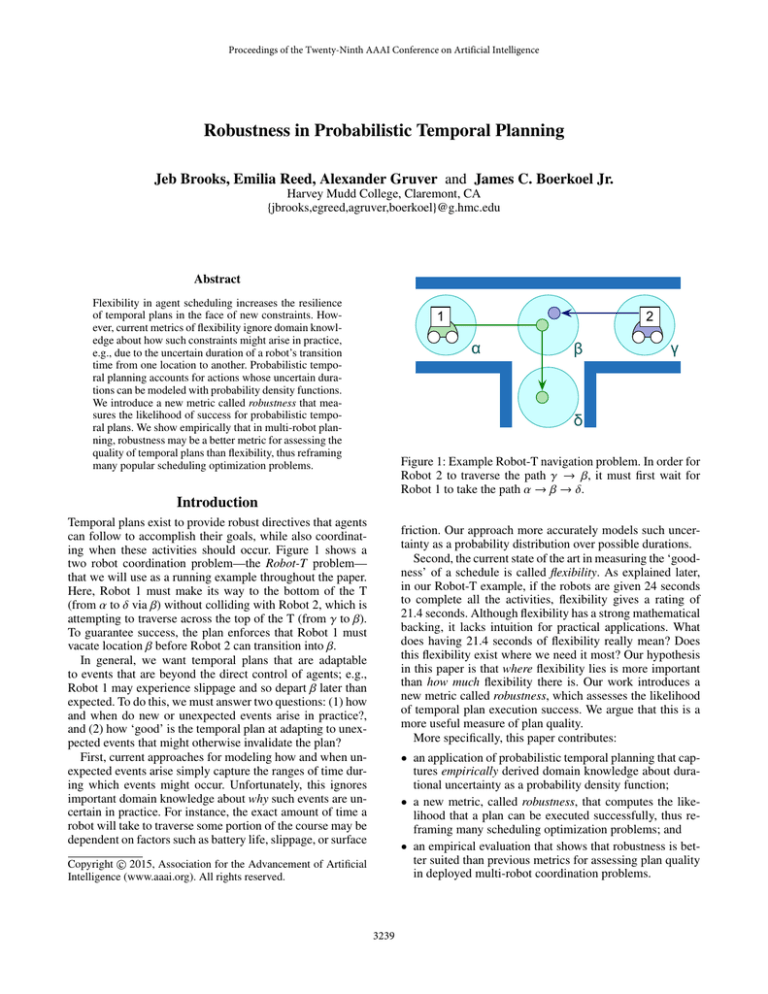
Figure 1: Example Robot-T navigation problem. In order for
Robot 2 to traverse the path γ → β, it must first wait for
Robot 1 to take the path α → β → δ.
Introduction
Temporal plans exist to provide robust directives that agents
can follow to accomplish their goals, while also coordinating when these activities should occur. Figure 1 shows a
two robot coordination problem—the Robot-T problem—
that we will use as a running example throughout the paper.
Here, Robot 1 must make its way to the bottom of the T
(from α to δ via β) without colliding with Robot 2, which is
attempting to traverse across the top of the T (from γ to β).
To guarantee success, the plan enforces that Robot 1 must
vacate location β before Robot 2 can transition into β.
In general, we want temporal plans that are adaptable
to events that are beyond the direct control of agents; e.g.,
Robot 1 may experience slippage and so depart β later than
expected. To do this, we must answer two questions: (1) how
and when do new or unexpected events arise in practice?,
and (2) how ‘good’ is the temporal plan at adapting to unexpected events that might otherwise invalidate the plan?
First, current approaches for modeling how and when unexpected events arise simply capture the ranges of time during which events might occur. Unfortunately, this ignores
important domain knowledge about why such events are uncertain in practice. For instance, the exact amount of time a
robot will take to traverse some portion of the course may be
dependent on factors such as battery life, slippage, or surface
friction. Our approach more accurately models such uncertainty as a probability distribution over possible durations.
Second, the current state of the art in measuring the ‘goodness’ of a schedule is called flexibility. As explained later,
in our Robot-T example, if the robots are given 24 seconds
to complete all the activities, flexibility gives a rating of
21.4 seconds. Although flexibility has a strong mathematical
backing, it lacks intuition for practical applications. What
does having 21.4 seconds of flexibility really mean? Does
this flexibility exist where we need it most? Our hypothesis
in this paper is that where flexibility lies is more important
than how much flexibility there is. Our work introduces a
new metric called robustness, which assesses the likelihood
of temporal plan execution success. We argue that this is a
more useful measure of plan quality.
More specifically, this paper contributes:
• an application of probabilistic temporal planning that captures empirically derived domain knowledge about durational uncertainty as a probability density function;
• a new metric, called robustness, that computes the likelihood that a plan can be executed successfully, thus reframing many scheduling optimization problems; and
• an empirical evaluation that shows that robustness is better suited than previous metrics for assessing plan quality
in deployed multi-robot coordination problems.
c 2015, Association for the Advancement of Artificial
Copyright Intelligence (www.aaai.org). All rights reserved.
3239
α1A
α
[1,2]
[0,24]
α1D
[0,24]
[4.6,∞)
β1A
β
[0,2]
[0,24]
β1D
[0,24]
[6.6,∞)
δ
1
δA
[0,24]
Robot 1
Robot 1
[0,24]
1
[1,2]
δD
[0,6.2]
α1A
α
[1,2]
[1,7.2]
α1D
[5.6,11.8]
[4.6,10.8]
β1A
γ
[1,∞]
[0,24]
γ 2D
[0,24]
[4.6,∞)
β2A
β
[1,2]
[0,24]
Robot 2
Robot 2
γ 2A
[0,2]
β1D
[12.2,18.4]
[6.6,12.8]
δ [13.2,20.4]
1
δA
1
[1,2]
δD
[0,6.2]
[0,∞)
[0,24]
β [5.6,11.8]
β2D
[0,17.4]
γ 2A
γ [12.2,18.4]
[1,18.3]
γ 2D
[16.8,23]
[4.6,10.8]
β2A
β [17.8,24]
[1,2]
β2D
Figure 3: Minimal (shortest path) version of Figure 2.
Figure 2: Temporal network corresponding to the Robot-T
problem. Each robot’s arrival (A) and departure (D) of a location is encoded as an event (timepoint), and all events must
occur between 0 and 24 seconds.
external constraints (Boerkoel and Durfee 2013).
The STN can be viewed as a constraint satisfaction problem, where each variable’s domain is defined implicitly
through constraints with the special zero timepoint, t0 ,
which represents the start of time and so is assumed to be
set to 0. Commonly, the domain of each timepoint is determined by a makespan constraint—the deadline between the
execution of the first and last events. From Figure 2, the fact
that γ2A has a domain of [0, 24] is encoded as γ2A −t0 ∈ [0, 24].
Solving an STN requires assigning a time to each timepoint
such that all temporal difference constraints are satisfied. A
feasible STN—one that has a solution—is called consistent.
As an alternative to a fully-assigned point solution, shortestpath algorithms such as Floyd-Warshall can be applied to an
STN’s distance graph in O(n3 ) time to compute a set of implied constraints. These implied constraints define minimal
intervals, which represent the sound and complete range of
times during which each event can take place. We display
minimal constraints for our running example in Figure 3.
Background
Figure 2 is a graphical representation of our Robot-T problem from the introduction. Each graph node is labeled
with the location it represents and a subscript that dictates
whether it is an arrival event (A) to or a departure event (D)
from that location. The constraint β1A − α1D ∈ [4.6, ∞), which
indicates that Robot 1 must take at least 4.6 seconds to traverse the distance from α to β (and has no maximum transit
time), is represented by the edge from α1D to β1A with label
[4.6, ∞). The constraint β1D − β1A ∈ [0, 2] represents that there
is no need for the robot to wait at location β as it passes
through, whereas the wait time at start/stop locations is at
least 1 second to allow for, e.g., a pick/drop activity. The fact
that each event in the Robot-T problem must be completed
within 24 seconds of the start of the task is represented by
the range of values [0,24] placed above each timepoint. Finally, which agent owns a particular timepoint is indicated
by superscript, where Robot 1’s subproblem is contained in
the top half of the figure, while Robot 2’s subproblem is contained in the bottom half of the figure. There is a single interagent (external) constraint, shown as a dashed line, which
dictates that Robot 1 must arrive at location δ (i.e., vacate
location β) before Robot 1 can depart location γ (to head
towards location β). This encoding of the Robot-T problem
is expressed as a Simple Temporal Network, a problem formalism we introduce next.
Quality of Simple Temporal Networks
A key to the popularity of the STN representation of temporal plans in real applications is that it naturally supports a flexible times representation (Bresina et al. 2005;
Barbulescu et al. 2010; Boerkoel et al. 2013). That is, when
the minimality of a temporal network is maintained the result is a space of all possible solutions. For instance, as
shown in Figure 3, Robot 1 can depart location α at any
time between 1 and 7.2 seconds. Thus, as new constraints
are introduced due to ongoing plan construction, execution,
or unexpected disturbances, as long as some of the feasible
schedules are retained, the integrity of the plan as a whole
remains intact. To fully exploit the advantages of the STN
we first need (1) a model to assess where new constraints
come from, and (2) a measure of an STN’s ability to adapt
to new constraints. Next we discuss related approaches that
address each of these needs and that inspire our approach.
Simple Temporal Networks
A Simple Temporal Network (STN), S = hT, Ci, is composed of T — a set {t0 , t1 , . . . , tn } of n + 1 timepoint variables, each of which represents a real-world event—and
C—a set of m temporal difference constraints, each of
which restricts the amount of time that can elapse between
two events and takes the form ci j := t j − ti ≤ bi j for some
real-value bounded bi j (Dechter, Meiri, and Pearl 1991). A
convenient graphical representation of an STN is called a
distance graph, where each timepoint is represented as a
vertex and each constraint t j − ti ≤ bi j is represented as an
edge from ti to t j with weight bi j . As a notational convenience, when ti − t j ≤ b ji also exists, the symmetric pair of
constraints involvingh ti and t ij can be combined into a single
constraint t j − ti ∈ −b ji , bi j . The Multiagent STN is one
that establishes how control of an STN is distributed among
agents as local subproblems that are related through a set of
STN with Uncertainty A Simple Temporal Network with
Uncertainty (STNU) partitions the set of constraints of an
STN into a set of requirement links and a set of contingent links (Vidal and Ghallab 1996). A requirement link is
a constraint that represents hard bounds on the difference between two timepoint variables. A contingent link, ki j , models the fact that the time that will elapse between ti and t j is
dictated by an uncontrollable process such as nature. Nature
will choose some value, βi j , between the specified lower and
upper bounds, t j − ti = βi j ∈ [−b ji , bi j ], which is unknown
3240
Robot 1
to the agent prior to execution. A contingent timepoint is
a timepoint t j that appears as the target of exactly one contingent link, ki j ; non-contingent timepoints are called executable. In Figure 2, an agent controls how much time it
spends at a location, but not the time it takes to navigate
between locations. Thus, all navigation constraints are contingent links (bold). A primary concern of the STNU literature is finding a controllable execution strategy—one that
guarantees success despite the presence of uncertain events,
our approach instead computes the likelihood of execution
success. While controllability is an extremely useful property, our approach aims to be useful in environments where
a plan is worth attempting even if success is not guaranteed,
e.g., when the expected value of attempting a plan may outweigh the costs of potential failure.
[0,0]
α1A
α
[1,2]
[1,2]
α1D
[6.6,8.6]
[4.6,7.6]
β1A
β
[0,2]
[8.6,8.6]
β1D
[15.2,16.2]
[6.6,7.6]
δ [17.2,17.2]
1
δA
1
[1,2]
δD
Robot 2
[0,22]
[0,15.2]
γ 2A
γ [16.2,17.4]
[1,17.4]
γ 2D
[22,23]
[4.6,6.8]
β2A
β
[1,2]
[24,24]
β2D
Figure 4: Interval schedule of the Robot-T Problem.
Wilson et al. propose a new flexibility metric that avoids
double counting by first decomposing all events into independent interval schedules. An interval schedule
h
i computes
− +
a range of times for each timepoint ti , ti , ti , such that
the execution of ti is independent of all other timepoints.
This is accomplished by enforcing that t+j − ti− ≤ bi j holds
for all constraints of the form t j − ti ≤ bi j , which guarantees
h
i that ti can be set to any value within its interval
ti− , ti+ without impacting the values to which t j can be set.
This allows
us to redefine the flexibility of a timepoint as
flex(ti ) = ti+ − ti− and the flexibility of a temporal network
P
as flex(S) = ni=1 flex(ti ), eliminating the concern that flexibility is over counted.
We present an interval schedule of our ongoing example
in Figure 4. Here, all assignments of times to timepoints that
respect the interval schedule will lead to a solution, since any
time within α1A ’s domain is guaranteed to be consistent with
any time within α1D ’s domain. As a result, the reported flexibility of the interval schedule drops from 73.2 seconds to
21.4 seconds. While flexibility yields an important measure
of scheduling slack, it may not tell the whole story.
Probabilistic STNs We originally proposed an extension
to STNUs that recognized that domain knowledge often exists to allow contingent links to be modeled more accurately
as probability density functions (pdf). We called this model
the STN with Modeled Uncertainty. However, Tsamardinos (2002) independently introduced a similar extension to
STNUs, called the Probabilistic Simple Temporal Network (PSTN), and so we have recast our contributions in
terms of this model for probabilistic temporal planning.
PSTNs augment STNUs’ definition of a contingent link
such that t j − ti = Xi j where Xi j is a random variable
that is determined by Pi j , a pdf that models the duration
of the link from ti to t j ; that is Xi j ∼ Pi j . This formulation of the PSTN permits the use of any distribution to describe the duration of an activity, including ones that are
parametrized, e.g. Pi j (S ). This means that any STNU can
be cast as a PSTN with uniform distributions over specified
ranges of times, making the PSTN strictly more expressive
than the STNU. Further, whenever it is possible to extract
bounds from the distributions used in a PSTN, any algorithm that establishes controllability for an STNU can still
be applied to a PSTN. Previous work has primarily focused
on generating execution strategies (assignments of times to
executable timepoints) that minimizes risk (i.e., maximizes
the likelihood of successful execution) (Tsamardinos 2002;
Fang, Yu, and Williams 2014)
A New Robustness Metric
Here we introduce a new metric called robustness for assessing the quality of probabilistic temporal plans. As motivation for how PSTNs can be applied to real-world problems,
consider the empirical distributions we captured (using the
experimental setup described later) for the time it takes our
robots to travel forward a single unit both with and without
completing a turn, labeled PT and PF respectively in Figure
5. Allowing the robot between 5.5 and 7.5 seconds to travel
forward, i.e., 2 seconds of flexibility, would lead to plan success (91.70% of the time) far more often than if the robot had
7.5 - 11.5 seconds, or 4 seconds of flexibility (which leads
to success only 6.02% of the time). That is to say, in realworld problems where uncertainty is controlled by a modelable process, where flexibility lies may often be more important than how much flexibility there is. In this section, we
formalize this idea of using models of durational uncertainty
to compute robustness, a measure of the likelihood of plan
success.
Flexibility of Temporal Networks Generally speaking,
the more schedules that a representation permits, the better
situated it is to adapt to new constraints as they arise. Wilson et al. (2014) formalized the idea of flexibility—a metric
that is designed to quantify the aggregate slack in temporal
plans. To parallel our later discussion about robustness, we
start by introducing the naı̈ve flexibility metric, flexN . The
flexN of a timepoint is the length of its domain interval, that
is flexN (ti ) = bi0 −(−b0i ), where ti −t0 ∈ [−b0i , bi0 ]. The flexN
of an entire temporal network, then,Pis the sum of the flexibility of its timepoints, flexN (S) = ni=1 flexN (ti ). The flexN
of the network in Figure 3 is 6.2 × 9 + 17.4 = 73.2 seconds.
This metric is naı̈ve in the sense that it systematically over
counts flexibility. For example, even though both α1A and α1D
have 6.2 seconds of flexibility, as soon as Robot 1 arrives at
location α, the flexibility of α1D shrinks to 1 (since it must
occur at least 1 and at most 2 seconds after α1A ).
Robustness of PSTNs
The PSTN problem formulation allows us to consider questions such as: How likely is a given temporal network to
3241
1.8
Forward Distribution PF
Turn Distribution PT
1.6
Algorithm 1: Sampling-based Simulator
1.4
PDF
1.2
1
1
0.8
2
0.6
3
0.4
4
0.2
5
0
-0.2
6
5
6
7
8
9
10
11
12
Input: A PSTN S , A number of samples N
Output: A robustness estimate for S
failures = 0
foreach i ∈ [1, N] do
while Not all timepoints have been assigned do
t = selectNextTimepoint(S )
if t ∈ ExecutableTimepoints then
t.assignToEarliestTime();
else
7
Time (s)
8
9
Figure 5: The empirical distributions for the robot transition
time of moving forward PF and turning PT one unit.
10
11
propagateConstraints(S )
if S is inconsistent then
failures += 1
break
12
13
lead to a successful execution? This is in contrast to previous STNU controllability algorithms, which presuppose (or
attempt to compute) a dispatch strategy that guarantees execution success. For many interesting problems, determining
a controllable execution strategy may be impossible, yet if
the likelihood of success is high enough, it might still be
worth attempting to execute the plan.
Our new robustness metric leverages domain knowledge
supplied within the PSTN definition to attempt to predict
the success rate of a given temporal plan. Our first attempt
at defining robustness, which we call naı̈ve robustness to
parallel our earlier discussion about naı̈ve flexibility, is:
Y Z ci j
Pi j (x)dx
c∈C
14
15
16
6.6
return 1 − (failures/N)
the likelihood of execution success (Tsamardinos 2002). To
correctly capture these inter-dependencies without committing to specific execution times for our running example, we
would need to construct a multi-dimensional integral that
adjusts the domain of integration the same way the network
updates the time intervals, for instance:
Z 10.8
Z 12.8−x
Z 10.8−(x+y)
PF (x)
PT (y)
PF (z)dz dy dx
−c ji
4.6
This metric is the product of the probability mass found
within contingent intervals specified in the PSTN. Applying
this metric to the network in Figure 3 yields:
Z 10.8
Z 12.8
Z 10.8
PF (x)dx ·
PT (x)dx ·
PF (x)dx
4.6
l = S .getContingentLink(t)
p = l.getPreviousTimepoint(t)
x = sample(Pl )
t.assign(p.getAssignedTime() + x)
6.6
4.6
While this multi-dimensional integral approach seems like
a promising way to compute the robustness of a temporal
network, it suffers from two fatal flaws. First, generally constructing and solving such systems of integrals quickly becomes intractable as the number of activities and complexity
of interdependencies grow. Second, as currently expressed,
the multi-dimensional integral approach implicitly assumes
that the agent gets to make all of its decisions after nature
has determined the duration of all contingent links, which is
of course not true in practice.
Next, we describe two computationally-efficient,
simulation-based methods that correct these shortcomings
by approximating the true robustness of temporal networks.
4.6
where PF and PT are the distributions from Figure 5.
The definition of a PSTN assumes that the pdfs that determine contingent links are independent from each other.
However, as noted in our discussion of the naı̈ve flexibility
metric, the time intervals within which these activities must
take place are not independent. Thus, our naı̈ve robustness
metric is overly optimistic for the same reason that the naı̈ve
flexibility metric over-counts slack.
As an example, if Robot 1 takes x seconds to travel from γ
to β, it will have x fewer seconds to travel from β to δ. Similarly, if it takes Robot 1 y seconds to from β to δ, Robot 2
will have (x + y) fewer seconds to complete its maneuver. So
to calculate the overall likelihood of success of a temporal
network requires evaluating every possible duration x that
an activity could take and weighting it by the likelihood of
future activities, given that the first activity took time x. Of
course, determining the likelihood of each subsequent activity relies recursively on its future activities, and vice-versa.
Previous approaches for predicting the likelihood of success for PSTNs have dealt with the problem of temporal
inter-dependencies by first assigning all executable timepoints, which makes contingent links temporally independent, but does so at the cost of unnecessarily decreasing
Sampling-based Simulator Approximation Our first approach for approximating the true robustness of a temporal
network is presented in Algorithm 1. Our Sampling-based
Simulator works by simulating N plan executions and counting the relative number of successes vs. failures. The selectNextTimepoint() function chooses timepoints in the same
order they would be executed in the plan. This is determined
using the next first protocol as defined by the dynamic controllability dispatcher (DC-dispatch), which always selects
timepoints that are both live (can occur next temporally)
and enabled (all incoming links have already been executed)
(Morris, Muscettola, and Vidal 2001).
If the selected timepoint is executable (has no incoming
contingent links), we follow the lead of DC-dispatch and assign to it the earliest possible time. Otherwise, if the selected
3242
timepoint is contingent, there must be exactly one incoming
contingent link. We extract that link, sample from its probability distribution to get a duration x, and then assign the
timepoint to occur x seconds after the previous timepoint’s
assigned time. If any assignment of a time to a timepoint
variable leads to an inconsistent network, we count the simulated plan execution as failure. Finally, after N iterations,
we return the overall success rate, (1 − (failures/N)).
Whereas
the
computationally-intractable
multidimensional integral approach theoretically evaluates
all possible combinations of contingent timepoint assignments, our Sampling-based Simulator instead draws sample
combinations according to their underlying likelihood. It
also captures temporal dependencies by propagating the
temporal implications of these samples to approximate
the frequency of success. Further, we faithfully recognize
that how nature chooses to assign contingent timepoints
only becomes known at execution time, and that, in the
meantime, agents must still choose how and when to
execute their executable timepoints, which we accomplish
by using the DC-dispatch strategy.
Our algorithm draws O(N) samples, where for each sample, each of O(|T |) timepoints is assigned and propagated using Floyd-Warshall, which takes O(|T |3 ) time. If we assume
that samples have been drawn as a preprocessing routine and
can be retrieved in constant time, the total runtime of our algorithm is O(N|T |4 ).
Our Representative Simulator (Algorithm 2) uses the
same basic dispatching method as our Sampling-based Simulator. The key idea is that as we simulate, we keep a running estimate of the robustness of the network, which is initially set to be 1.0 (i.e., 100% likely). Then, before we assign a contingent timepoint, we first calculate the probability
mass that lies within its current temporal bounds and multiply this probability into our running estimate. Next, we use
the selectTime function to select a time that both lies within
the bounds specified and is representative of the underlying
distribution. This ensures that we will evaluate a complete,
representative simulation. In our implementation of the algorithm, we use the expected value to act as the representative
sample, but any metric, such as median or mode, could be
substituted. The rationale for our approach is that assigning
a timepoint effectively decomposes it from the rest of the
schedule, which eliminates temporal dependencies between
contingent links and so allows us to multiply the probabilities together as a running product.
We now demonstrate how Representative Simulator
works on a small portion of our running Robot-T example.
First, it fixes points γ2A and α1A to their minimum value of 0,
since they have no incoming edges from unassigned timepoints. This makes the timepoint α1D enabled, and because
its only incoming edge is a requirement edge, it also gets
assigned its minimum value of 1. Next the algorithm will
compute the robustness of the edge α1D → β1A . This edge has
constraints [4.6, 10.8] and so the algorithm will calculate the
probability of success of that edge as:
Z 10.8
pα1D ,β1A =
PF (x)dx = 1.0
Representative
Simulator
Approximation Our
Sampling-based Simulator may require a large number
of iterations to accurately approximate the robustness of the
underlying temporal network. For cases where efficiency
is a primary concern, we have devised another simulationbased algorithm that approximates the robustness of a
temporal network in a single pass. The idea is that, when
we select a duration for a contingent link, instead of generating a random sample, we instead select a representative
sample—one that acts as a proxy for the various ways the
random samples could play out.
4.6
which happens to capture its entire probability mass. The
expected value is then computed:
Z 10.8
x × PF (x)
eα1D ,β1A =
dx = 6.12
pα1D ,β1A
4.6
Next the algorithm sets the timepoint β1A to α1D + eα1D ,β1A =
7.12. The algorithm then propagates the new constraints and
repeats this process for all remaining timepoints.
The runtime of this algorithm is O(|T |(|T |3 + I)) where I is
the runtime of the integrator. However, its accuracy depends
on how well the choice of representative sample approximates the convolution of distributions.
Algorithm 2: Representative Simulator
1
2
3
4
5
6
7
8
9
10
11
12
13
14
Input: A PSTN S
Output: A robustness estimate for S
robustness = 1.0
while Not all timepoints have been assigned do
t = selectNextTimepoint(S )
if t ∈ ExecutableTimepoints then
t.assignToEarliestTime();
else
Empirical Evaluation
With our two new robustness approximations in hand, we
now ask how well these metrics assess the quality of temporal plans in a deployed multi-robot navigation scenario.
l = S .getContingentLink(t)
p = l.getPreviousTimepoint(t)
R lmax
prob = l
Pl (x)dx
min
robustness = robustness × prob
x = selectTime(Pl , lmin , lmax )
t.assign(p.getAssignedTime() + x)
Experimental Setup
Our experiments involved iRobot Creates performing simple navigation tasks. We placed two brightly colored markers on top of each robot and monitored these markers with a
Microsoft Kinect in order to track the location and orientation of the robots. Using this information, we built a simple
propagateConstraints(S )
return robustness
3243
23
1
70
22
0.8
65
21
0.8
19
18
0.4
17
0
16
Empirical Robustness
Naive Robustness
Sampling Simulator
Representative Simulator
Flexibility
0.2
18
19
20
21
22
Makespan Time (s)
23
24
Robustness (%)
0.6
Flexibility (s)
Robustness (%)
20
15
60
55
0.6
50
0.4
45
Empirical Robustness
Naive Robustness
Sampling Simulator
Representative Simulator
Flexibility
0.2
14
25
13
0
28
30
32
34
Makespan Time (s)
36
38
Flexibility (s)
1
40
35
40
30
Figure 6: Comparison of our robustness approximations
against both experimental data and flexibility for the RobotT experiment.
Figure 7: Comparison of our robustness approximations
against both experimental data and flexibility for the RobotPass experiment.
control system that enabled the robots to accurately navigate
from point to point on a grid.1
We focused our efforts on the Robot-T and Robot-Pass
experiments. The Robot-Pass experiment involves three
robots and three unique points of coordination.2 For each of
these experiments, we varied the makespan deadline within
which the robots had to complete the entire navigation
plan. In all of our experiments, we dispatched robots using the DC-dispatch protocol (described above) and used
DI∆STP (Boerkoel et al. 2013), a distributed algorithm
that exploits multiagent structure as our implementation of
propagateConstraints(S ). To generate the Empirical Robustness curve in the charts below, we ran each multi-robot scenario 50 times for each deadline. For each run, we recorded
whether or not the robots successfully completed the navigation plan within the allotted time.
For the two approximation algorithms, we used the PF
and PT pdfs displayed in Figure 5 as our models of durational uncertainty for the PSTN input to both the Samplingbased Simulator (N = 1000) and Representative Simulator. We empirically derived these pdfs by running our three
robots around a one unit square 100 times each, and for each
independent maneuver, building a histogram using a kernel
smoother. Finally, we also report the output of both our naı̈ve
robustness metric and Wilson et al.’s flexibility metric computed with PuLP, a Python library that leverages CoinMP an open source linear programming library.
of robustness—the robots succeeded more often in the realworld than our PSTN model would predict. Our preliminary
explorations indicate that this is due to the fact that, in practice, the underlying distributions are not independent, as is
assumed by our PSTN model. In fact, correlations may be
both positive—a robot that is running fast in the first leg of
the experiment is more likely to run fast in the second leg—
and negative—a robot that ‘arrives’ faster by getting acceptably close to its target (within its spatial tolerance) in the
first leg may require further adjustment in the second leg.
There are also differences between the shape of our two
robustness approximations. While our sampling-based simulation attempts to directly mimic the real-world scenario
using many sample executions, the representative-based
sampling method attempts to predict this value in one shot.
Differences between the two are due to the fact that combining the expected values of various distributions (representative) is not the same as the expectation of their convolution
(sampling-based). Flexibility tends to grow linearly with the
experimental deadline, indicating no obvious connection between a plan’s flexibility and chance of success.
The two algorithms also exhibit slightly different runtime behavior. We tested our algorithms on an Intel Xeon
E5-1603 2.80GHz quadcore processor with 8 GB of RAM
running Ubuntu 12.04 LTS. The runtime results reported in
Figure 8 are the average execution time across 20 executions of each configuration. We found that at low makespans,
the Sampling-based simulator can fail early in its simulation and so has relatively short runtime. Additionally we see
that the sampling simulator grows linearly with N, each time
the number of samples is doubled the run time doubles. Because the Representative simulator is making a sub-process
call to the Mathematica-based integrator, it does not recieve
the same benefits from early failure. Surprisingly, we found
that the Representative simulator performs similarly to the
Sampling-based simulator set at N = 1000, which was the
setting we found to perform well. It is important to note that
the sampling simulator is embarrassingly parallel and thus
can benefit from parallelization, whereas the representative
simulator cannot. Thus, further work is needed to better assess the computational trade-offs of these two approaches as
the scale and complexity of problems grows.
Analysis
Figures 6 and 7 show each of the aforementioned curves for
the Robot-T and Robot-Pass experiments, respectively. In
general, the increased size and complexity of the Robot Pass
problem yielded more variance in our results. In both experiments, the shape of our robustness curves more closely
matches the empirically measured success rate than either
the flexibility or naı̈ve robustness metrics.
As predicted, the naı̈ve robustness calculation is overly
optimistic. Surprisingly, both our Sampling-based and Representative approaches are pessimistic in their predictions
1
2
Control code available upon request.
Video available at: http://tinyurl.com/ocslka7
3244
Representative Simulator
Sampling (N=2000)
Sampling (N=1000)
Sampling (N=500)
Sampling (N=250)
7
Robustness (%)
Run Time (s)
6
5
4
3
0.16
28
0.14
26
0.12
24
0.1
22
0.08
20
0.06
18
2
0.04
1
0.02
0
0
18
19
20
21
22
Makespan (s)
23
24
25
Figure 8: Algorithm runtimes for the Robot-T experiment.
Flexibility (s)
8
16
14
Representative Simulator
Flexibility
18
20
22
24
Makespan Time (s)
26
28
30
12
Figure 9: Comparison of robustness and flexibility as applied
to an interval schedule version of the Robot-T experiment.
Finally, let us consider our earlier hypothesis that having flexibility in the right places matters more than having
more flexibility. We tested this hypothesis by approximating
the robustness of interval schedules for the same Robot-T
problem presented in Figure 6. As a reminder, the process
of computing interval schedules artificially constrains timepoints into temporally independent intervals so that flexbility is not double counted. However, if all that matters
is the total flexibility, we would expect that removing redundant slack from the schedule would have no impact on
robustness. We modified Wilson et al.’s approach to computing interval schedules, because initially our LP-solver
would return interval schedules that provided no slack to
one or more contingent timepoints (which yields a 0% success rate). Our modification replaced the objective function
of the LP-formulation so that it prioritized contingent timepoints (since executable timepoints are chosen by agents and
so require no flexibility). The results are shown in Figure 9.
Notice that despite the steady increase in flexibility, the
robustness of the PSTN does not continue to increase. In
fact, as the makespan increases to beyond 24 seconds, there
is a decrease in robustness. The reason is that even though
the size of the intervals increase as flexibility increases, the
location of the intervals also shifts towards the tail of the
distribution. So even though flexibility is increasing in absolute terms, the intervals are capturing less of the probability mass, thus decreasing robustness. Interestingly, this data
also appears to refute Wilson et al.’s conjecture that computing an interval schedule has no costs in terms of flexibility.
In other words, while flexibility correctly measures scheduling slack, it does not provide practical insight into a plan’s
adaptability in real world problems. This argues for reframing many scheduling optimization problems in terms of robustness rather than flexibility.
mate plan success rate than previous metrics for determining
the quality of a schedule. Robustness provides a supplement
to, not a replacement for, controllability—robustness provides helpful information for determining whether or not a
plan is worth attempting (in expectation) even if agents cannot completely hedge against uncertainty.
This paper provides many future research directions.
First, we would like to improve the quality of our robustness approximations and better understand the theoretical implications of the assumptions that PSTNs make (primarily that the pdfs representing durational uncertainty are
independent). Second, assessing the robustness and flexibility of solution methods is hardly a new idea in AI.
For instance, both ideas have been explored in the context of finite-domain constraint programming for dynamic
and uncertain environments (Verfaillie and Jussien 2005;
Climent et al. 2014). An interesting future direction inspired
by this literature is exploring whether the ideas of reactive
approaches, which try to repair a broken schedule with minimal upheaval, or proactive approaches, which try to use
knowledge about possible future dynamics to minimize their
effects, are better suited for the continuous nature of temporal planning. Finally, perhaps the most interesting future
research direction is in reframing scheduling optimization
problems in terms of robustness, rather than flexibility. As
demonstrated in this paper, simply maximizing flexibility
fails to produce robust schedules (see Figure 9). Interesting
optimization problems include computing optimal temporal
decouplings of multiagent schedules (Planken, de Weerdt,
and Witteveen 2010), and controllable schedules (Wilson et
al. 2014). One challenge is that the efficiency of previous
optimization approaches has relied on the linearity of flexibility as a metric, whereas optimizing for robustness requires
accounting for non-linear distributions; however the payoff
is that we will have plans that are more robust to the messiness of the real-world.
Conclusion
In this paper, we employ probablistic temporal planning as a
way to more precisely capture the nature of scheduling uncertainty within real-world problems. We developed a new
metric for assessing the quality of probabilistic temporal
plans called robustness. Our robustness metric utilizes the
model of durational uncertainty to estimate the likelihood of
success of a given temporal plan. Our empirical evaluation
demonstrates that our robustness approximations better esti-
Acknowledgements
We would like to thank Melissa O’Neill, Susan Martonosi,
Jacob Rosenbloom, Priya Donti, and the anonymous reviewers for their helpful feedback.
3245
References
Barbulescu, L.; Rubinstein, Z. B.; Smith, S. F.; and Zimmerman, T. L. 2010. Distributed coordination of mobile
agent teams: The advantage of planning ahead. In Proc. of
AAMAS-10, 1331–1338.
Boerkoel, J. C., and Durfee, E. H. 2013. Distributed Reasoning for Multiagent Simple Temporal Problems. Journal
of Artificial Intelligence Research (JAIR) 47:95–156.
Boerkoel, J. C.; Planken, L. R.; Wilcox, R. J.; and Shah, J. A.
2013. Distributed algorithms for incrementally maintaining
multiagent simple temporal networks. In Proc. of ICAPS-13,
11–19.
Bresina, J.; Jónsson, A. K.; Morris, P.; and Rajan, K. 2005.
Activity planning for the Mars exploration rovers. In Proc.
of ICAPS-05, 40–49.
Climent, L.; Wallace, R. J.; Salido, M. A.; and Barber, F.
2014. Robustness and stability in constraint programming
under dynamism and uncertainty. J. Artif. Intell. Res.(JAIR)
49:49–78.
Dechter, R.; Meiri, I.; and Pearl, J. 1991. Temporal constraint networks. In Knowledge Representation, volume 49,
61–95.
Fang, C.; Yu, P.; and Williams, B. C. 2014. Chanceconstrained probabilistic simple temporal problems. In
Proc. of AAAI-14, 2264–2270.
Morris, P.; Muscettola, N.; and Vidal, T. 2001. Dynamic
control of plans with temporal uncertainty. In Proc. of
IJCAI-01, 494–502.
Planken, L. R.; de Weerdt, M. M.; and Witteveen, C. 2010.
Optimal temporal decoupling in multiagent systems. In
Proc. of AAMAS-10, 789–796.
Tsamardinos, I. 2002. A probabilistic approach to robust
execution of temporal plans with uncertainty. In Methods
and Applications of Artificial Intelligence. Springer. 97–108.
Verfaillie, G., and Jussien, N. 2005. Constraint solving in
uncertain and dynamic environments: A survey. Constraints
10(3):253–281.
Vidal, T., and Ghallab, M. 1996. Dealing with uncertain
durations in temporal constraint networks dedicated to planning. In Proc. ECAI-96, 48–54.
Wilson, M.; Klos, T.; Witteveen, C.; and Huisman, B. 2014.
Flexibility and decoupling in simple temporal networks. Artificial Intelligence 214:26–44.
3246