Proceedings of the Twenty-Ninth AAAI Conference on Artificial Intelligence
Risk Based Optimization for Improving Emergency Medical Systems
Sandhya Saisubramanian and Pradeep Varakantham and Hoong Chuin Lau
School of Information Systems, Singapore Management University
80 Stamford Road, Singapore 178902
{sandhyas, pradeepv, hclau}@smu.edu.sg
Abstract
In emergency medical systems, arriving at the incident location a few seconds early can save a human life. Thus, this
paper is motivated by the need to reduce the response time
– time taken to arrive at the incident location after receiving
the emergency call – of Emergency Response Vehicles, ERVs
(ex: ambulances, fire rescue vehicles) for as many requests as
possible. We expect to achieve this primarily by positioning the ”right” number of ERVs at the ”right” places and at
the ”right” times. Given the exponentially large action space
(with respect to number of ERVs and their placement) and the
stochasticity in location and timing of emergency incidents,
this problem is computationally challenging. To that end, our
contributions building on existing data-driven approaches are
three fold:
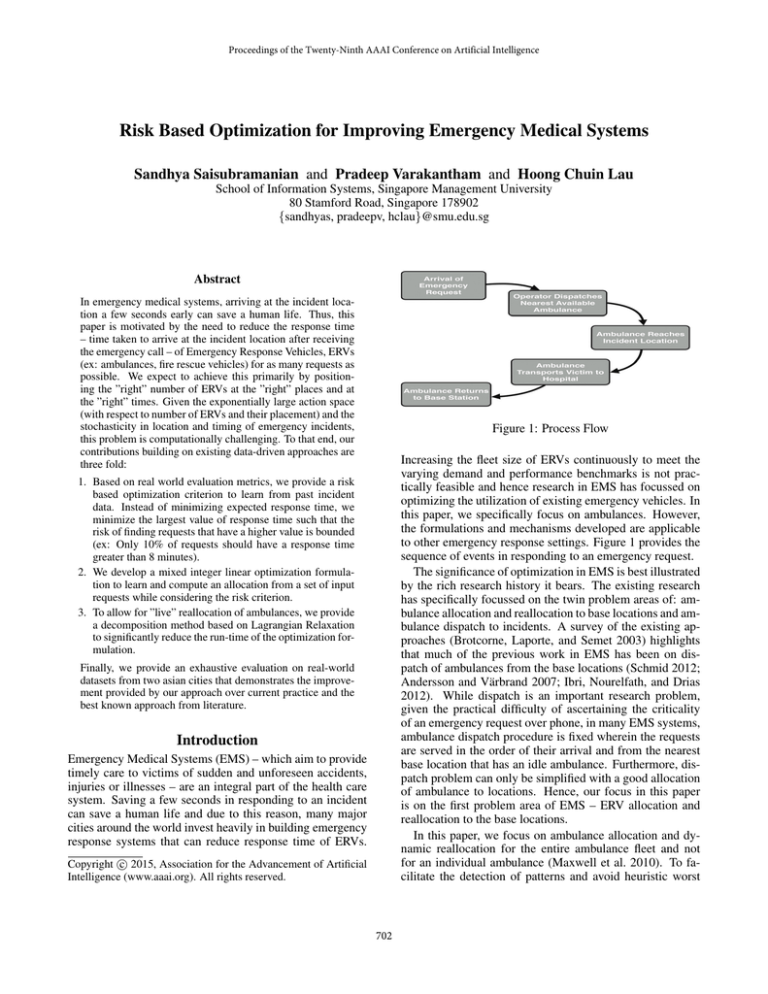
Figure 1: Process Flow
Increasing the fleet size of ERVs continuously to meet the
varying demand and performance benchmarks is not practically feasible and hence research in EMS has focussed on
optimizing the utilization of existing emergency vehicles. In
this paper, we specifically focus on ambulances. However,
the formulations and mechanisms developed are applicable
to other emergency response settings. Figure 1 provides the
sequence of events in responding to an emergency request.
The significance of optimization in EMS is best illustrated
by the rich research history it bears. The existing research
has specifically focussed on the twin problem areas of: ambulance allocation and reallocation to base locations and ambulance dispatch to incidents. A survey of the existing approaches (Brotcorne, Laporte, and Semet 2003) highlights
that much of the previous work in EMS has been on dispatch of ambulances from the base locations (Schmid 2012;
Andersson and Värbrand 2007; Ibri, Nourelfath, and Drias
2012). While dispatch is an important research problem,
given the practical difficulty of ascertaining the criticality
of an emergency request over phone, in many EMS systems,
ambulance dispatch procedure is fixed wherein the requests
are served in the order of their arrival and from the nearest
base location that has an idle ambulance. Furthermore, dispatch problem can only be simplified with a good allocation
of ambulance to locations. Hence, our focus in this paper
is on the first problem area of EMS – ERV allocation and
reallocation to the base locations.
In this paper, we focus on ambulance allocation and dynamic reallocation for the entire ambulance fleet and not
for an individual ambulance (Maxwell et al. 2010). To facilitate the detection of patterns and avoid heuristic worst
1. Based on real world evaluation metrics, we provide a risk
based optimization criterion to learn from past incident
data. Instead of minimizing expected response time, we
minimize the largest value of response time such that the
risk of finding requests that have a higher value is bounded
(ex: Only 10% of requests should have a response time
greater than 8 minutes).
2. We develop a mixed integer linear optimization formulation to learn and compute an allocation from a set of input
requests while considering the risk criterion.
3. To allow for ”live” reallocation of ambulances, we provide
a decomposition method based on Lagrangian Relaxation
to significantly reduce the run-time of the optimization formulation.
Finally, we provide an exhaustive evaluation on real-world
datasets from two asian cities that demonstrates the improvement provided by our approach over current practice and the
best known approach from literature.
Introduction
Emergency Medical Systems (EMS) – which aim to provide
timely care to victims of sudden and unforeseen accidents,
injuries or illnesses – are an integral part of the health care
system. Saving a few seconds in responding to an incident
can save a human life and due to this reason, many major
cities around the world invest heavily in building emergency
response systems that can reduce response time of ERVs.
c 2015, Association for the Advancement of Artificial
Copyright Intelligence (www.aaai.org). All rights reserved.
702
case planning (Andersson and Värbrand 2007), we employ
a data-driven approach, similar to the work by (Yue, Marla,
and Krishnan 2012). Ironically, even though target metrics and actual evaluation of EMS are based on the notion of bounded risk (Hong Kong 2009; Australia 2013;
Ontario 2013; Singapore 2013; Wales 2014; NFPA 2010),
researchers have focussed on optimizing other metrics such
as expected response time (Yue, Marla, and Krishnan 2012;
Schmid 2012). We address this discrepancy by considering
the risk based optimization criterion and that is also the main
distinction from existing work.
In addition to the greedy mechanism1 by (Yue, Marla,
and Krishnan 2012), existing work has provided heuristic
search based mechanisms for computing allocation (Gendreau, Laporte, and Semet 2001) based on modelling as a
coverage problem. On the contrary, we focus on a scalable
approximation approach with guarantees on learned allocation to learn from past data. To that end, our main contribution is an optimization formulation that provides novel insights on enforcing resource capacity constraints for a continuous time line using scalable linear constraints. Furthermore, by employing intuitions from Sample Average Approximation (Pagnoncelli, Ahmed, and Shapiro 2009), we
enforce the risk constraint using discrete variables and a linear constraint. In order to achieve scalability that will assist
in live decision support, we also develop a partition technique based on Lagrangian relaxation.
We evaluate the effectiveness of our techniques on realworld ambulance data sets from two large cities in Asia. The
experimental results show that in addition to outperforming
the best known approach in the literature (Yue, Marla, and
Krishnan 2012), our approach is able to reduce the response
time by at least a few minutes over current practice.
that the percentage of requests exceeding that response time
is less than the tunable input paramater, α. We refer to this
response time as the α-response time. Since a request can
be served from more than one base locations, the MILP formulation to determine the ”right” allocation of ambulances
to base locations such that the α-response time is reduced,
becomes challenging.
MILP formulation for Ambulance Allocation
We now provide a Mixed Integer Linear Program (MILP)
formulation for ambulance allocation. A detailed discussion
on major assumptions made in the formulation and how they
can be relaxed are presented in the latter section. Table 1
provides the variables and constants that are employed in
the formulation.
The goal of the linear formulation is to minimize a response time value δ by addressing the following challenges:
1. Ensuring that the probability of exceeding δ is
bounded by α: This is a chance constraint:
P r(δ r ≥ δ) ≤ α
r
where δ is the response time for request r and probability
is computed over the set of requests R.
Insight 1 Since we have a discrete set of requests, we can
use the technique adopted in Sample Average Approximation (SAA) (Pagnoncelli, Ahmed, and Shapiro 2009;
Varakantham and Kumar 2013) to provide an equivalent
set of linear constraints as follows:
δr − δ
,
∀r ∈ R
(1)
z r ∈ {0, 1} , z r ≥
M
r
rz
≤α
(2)
|R|
It should be noted that the variable z r is set to 1 if δ r
is greater than δ and 0 otherwise. Therefore, sum of all
z r variables divided by total number of requests gives the
percentage and hence should be less than α.
2. Computing available ambulances at each location l, at
the point of arrival of request r:
Motivation: Ambulance Allocation
Formally, ambulance allocation problem for a given set of
requests is given by the tuple:
R, B, A, T, C, α
The set of emergency requests is given by R and any
emergency request, r in R is defined as the tuple t, s, h,
where t is the arrival time, s is the source location of the
emergency and h is the nearest hospital to serve the request.
The set of base locations is given by B and the set of ambulances is given by A. T is a two dimensional vector providing the time taken to travel between any two locations in the
city and this information is typically obtained from mapping
services like google maps. More specifically, Tl1 ,l2 is the
time taken to travel from l1 to l2 . Cl provides the maximum
number of ambulances that can be stationed at base location
l.
The goal is to compute an allocation, a of ambulances to
base locations, that has the least value of response time, such
Insight 2 Since the set of requests are known before
hand, by computing binary constants, Flq,r , we can compute number of available ambulances using a linear constraint on the binary variables y as shown in Equation 3.
ylq · Flq,r , ∀r ∈ R, l ∈ B
(3)
arl = al −
q∈R,q.t<r.t
Variables/
Constants
al
arl
ylr
Flq,r
1
Unlike for expected response time objective (Yue, Marla, and
Krishnan 2012), the learning problem for a given set of requests
when optimizing with bounded risk notion is not sub-modular.
Hence, greedy mechanism is also a heuristic and does not provide
any quality guarantees.
Definition
Number of ambulances at l
Number of ambulances at l when r arrives
Binary variable that indicates if request r is
served by an ambulance from l.
Binary constant indicating whether an ambulance at l, if deployed to serve request q, will
be available to serve the next request r
Table 1: Notation
703
arl ≥ 0, ∀r ∈ R, l ∈ B
al ≤ Cl , ∀l ∈ B
al = |A|
(4)
(5)
(6)
l
For each location, constraint 3 computes the number of
idle ambulances based on the number of ambulances still
serving previous requests(second part of right hand side)2 .
Constraints 4,5,6 ensure number of ambulances is a whole
number and is within the capacity of the location, while
also preventing any violation of the fleet size.
3. Preventing service of a request when there are no ambulances available: This is achieved by using a logical
constraint that sets ylr variables for all locations to be zero.
ylr = min(1,
l
arl ),
∀r ∈ R
Figure 2: Partition of requests on a real request set
requests for those 4 hours on multiple different days in creating the request set. Hence, all these requests over different days are naturally independent. In the more interesting
case of static allocation, there may not exist an exact partition across days. Figure 2 provides a small example of
requests (taken from data set) and their connectivity (obtained from F). In such cases, we adopt minimal separator
algorithm (Shen and Liang 1997) to provide the partitions
and correspondingly get the number of requests to be removed. In the example of Figure 2, we had to remove 12%
requests to obtain the two partitions. Even though we remove requests, it is possible to maintain the risk bound of
the original problem and obtain a conservative estimate of
the optimal α response time by increasing the risk bound to
α + 4 , where corresponds to the percentage of requests
that are removed. This provides a conservative estimate, because we assume that all % of requests will have a response
time higher than the optimal in the original.
An updated optimization corresponding to partitions, ξ is:
(7)
l
4. Computing response time given y variables: We can
only ensure that the response time has a lower bound
using the following constraint. However, in conjunction
with objective and bounded risk constraint, response time
for every request is equivalent to the lower bound.
δr ≥
l
(ylr · Tl,r.s ) + (1 −
ylr ) · M
∀r ∈ R
(8)
l
Constraints 1-8 along with an objective of ”mina δ” form
the complete MILP. Henceforth, we refer to the response
time δ, as α-response time for the given set of requests, R.
Partitioning the Request Set for Scalability
The computational complexity of the MILP introduced in
the previous section increases rapidly with increase in the
number of requests (Figure 6). To counter this computational complexity, we exploit the notion of independence
among requests. A formal definition of dependence of requests is presented below using the binary vector, F.
Definition 1 Two requests q and r are dependent if there
exists at least one location l for which Flq,r = 1.
The dependency between requests is with respect to being
served by an ambulance from the same base location. We
pursue a two step approach to identify and exploit independence between requests:
1. Identify the minimum set of requests, say G in the request
set R, that if removed can create ξ independent partition
sets of the request set with ∪k≤|ξ| ξk = R \ G
2. Given the independent partitions and the new set of requests R \ G, we compute one ambulance allocation
(and not one ambulance allocation for each partition)
that works across the independent partitions by using the
well known technique of Lagrangian dual decomposition(LDD) (Fisher 1985)3 .
For (1), in the case of dynamic reallocation of ambulances
for a small interval of time (say 4 hours), we only consider
min
δk
k≤|ξ|
s.t. P r(δkr ≥ δk ) ≤ α + ,
arl,k = al,k −
∀r ∈ ξk , k ≤ |ξ| (9)
q
yl,k
·
r,q
Fl,k
,
∀r, k, ∀l ∈ B
(10)
∀l
(11)
∀k
(12)
∀r, l, k
(13)
∀r, k
(14)
ylr ) · M, ∀r, k
(15)
q∈ξk ,q.t<r.t
al,k ≤ Cl ,
al,k = |A|,
l
aql,k
≥ 0,
r
yl,k
l
δkr ≥
= min(1,
arl,k ),
l
r
(yl,k
· Tl,r.s ) + (1 −
l
al,k = nl , ∀k, l
l
(16)
In the above optimization problem, we employ nl to ensure
all partitions have the same allocation of ambulances. Constraint 16 ensures that allocations across partitions are equal.
Dual Decomposition—————–
Except for constraint 16, all the other constraints are defined
2
4
Please refer to supplementary file for steps to compute F value.
Please refer to the supplementary material for a background on
Lagrangian dual decomposition.
It should be noted that there may be no solution once the risk
value is increased to account for the removed requests. In such a
case, we can only get a heuristic approximation with this algorithm.
3
704
min δk
s.t. P r(δkr ≥ δk ) ≤ α + ,
arl,k = al,k −
∀r ∈ ξk
q
yl,k
·
r,q
Fl,k
,
allocation, Ak for a partition q is obtained by replacing all
occurrences of al,q with Al,k in S OLVE S LAVE(q);
Algorithm 1 provides the pseudo code for the overall procedure of Lagrangian dual decomposition. We stop our lagrangian approach when the duality gap (difference between
the primal and dual value) falls below a tunable value,μ.
(19)
∀r, ∀l ∈ B (20)
q∈ξk ,q.t<r.t
al,k ≤ Cl ,
al,k = |A|
l
aql,k
∀l
r
yl,k
= min(1,
δkr ≥
Algorithm 1: SolveLDD()
0
1 Initialize: λ , it ← 0 ;
2 repeat
3
∀k : dk , Ak ← S OLVE S LAVE(k)
4
Update prices according to Equation 18
5
p, Ap ← E XTRACT P RIMAL ({Ak }k≤|ξ| );
6
it← it + 1;
7 until p −
k≤|ξ| dk ≤ μ;
8 return p, Ap
(22)
≥ 0,
l
(21)
∀r, l (23)
arl,k ),
l
r
(yl,k
· Tl,r.s ) + (1 −
l
∀r
(24)
ylr ) · M, ∀r
(25)
l
Table 2: S OLVE S LAVE(k)
on a specific partition. Hence, we obtain the Lagrangian by
dualizing constraint 16:
L(λ) = min
ak ,n
δk +
Dynamic Reallocation
λl,k · (al,k − nl )
When there exists a strong pattern of requests coming
through in a few hours, it is beneficial to alter the allocation computed from a large set of requests. For instance, on
a wednesday or friday night, there is high chance of emergency events occuring near areas with clubs as there are
large gatherings of people due to ladies’ night or weekend.
By using request sets for the next few hours from multiple
days, S OLVE LDD() can be used to obtain a new allocation.
While such a modification is applicable, there are practical
concerns: (a) only a few ambulances are available for allocation at that time step; and (b) ambulances could spend
a significant time moving between base locations without
serving requests.
Therefore, we consider reallocating ambulances by minimizing movements with respect to existing allocation of ambulances. This ensures that many ambulances do not remain
unavailable for long while undergoing reallocation. We introduce a penalty parameter p, that is calculated as the difference between the orginal allocation and the planned reallocation. This penalty paramater helps to keep a check
on drastic changes to the existing allocation and to ensure
better α-response time with minimal movement of ambulances. Users can adjust the input parameter Γ which serves
as upper bound for the penalty parameter p, to balance performance and reallocation of the fleet. We add the following
constraints to achieve the reallocation with minimal movement. al denotes the number of ambulances at l, obtained
by previous allocation and nl denotes the number of ambulances at l after reallocation.
(nl − al ); p ≤ Γ
(26)
p=
l,k
k≤|ξ|
or alternatively
= min
a
δk +
λl,k · al,k ) − min
λk,l · nl
n
l
k≤|ξ|
k≤|ξ|,l
Since nl is unbounded, the overall optimization will be unbounded.
The equivalent bounded optimization for calculating L(λ) is:
δk +
λl,k · al,k ) s.t.
λk,l = 0, ∀l (17)
min
a
l
k≤|ξ|
k≤|ξ|
If we use an update rule for λ that ensures the constraint 17
is always satisfied, then L(λ) decomposes over the individual partitions. Table 2 provides the slave optimization
problem corresponding to each partition k.
Update of Price Variables—————–
In order to ensure that dualized constraint violations
are minimized, the final optimization at the master is:
maxλ L(λ) and we solve this optimization using subgradient descent on λ. Combining the update required for
sub-gradient descent and for satisfaction of constraint 17,
we have the following update rule:
t+1
λt+1
l,k = λ̃l,k −
k
λ̃t+1
l,k
t+1
t
t
t+1 && λ̃l,k = λl,k + γ · al,k (18)
λ̃
k l,k
Primal Extraction from Dual Solution, {Ak }k≤|ξ| ——
Let the dual solution values be {Ak }k≤|ξ| , once all the slave
optimization problems are solved. When the ambulance allocations across the partitions are not equal, the obtained
dual solution is not a feasible primal solution. However, all
the following derived allocations are feasible solutions given
the dual solution: A1 , A1 , · · · , A1 , A2 , A2 , · · · , A2 , . . ..
Amongst all these solutions, we take the one which provides
the least value of α-response time as the primal solution for
the current iteration. α-response time for a given ambulance
l
Experimental Results
We perform experiments on real world data by varying parameters to make the following performance comparisons:
• Risk based optimization (RBO) and the current practice
(response time observed from the data).
705
(b) α response time comparison
(a) Results on multiple test sets
Figure 3: RBO Vs Current practice
(a) Dataset1: Effect of fleet size (b) Dataset2: Effect of fleet size
(c) Dataset1: Effect of α
(d) Dataset2: Effect of α
Figure 4: RBO Vs Greedy approach
• RBO and the best known approach for ambulance allocation in the literature(Yue, Marla, and Krishnan 2012).
obtained allocation, we use the standard dispatch technique,
wherein a request that arrives first is serviced and by an
available ambulance nearest to the incident location. Unless
otherwise stated, the default settings of the experiments are
α = 0.2, fleet size of dataset1 = 40 and fleetsize of datatset2
= 58. The experiments involving RBO refer to RBO with
LDD.
• RBO with and without LDD.
• Dynamic reallocation and static allocation.
We experiment with two data sets, namely Dataset1 and
Dataset2 obtained from two asian cities. Dataset2 is adopted
from (Yue, Marla, and Krishnan 2012). Both these datasets
provide information about emergency requests over a sustained period of time (1 year). An emergency request consists of the time of request arrival, incident location and
hospital location for the request. We also have information about number of ambulances, categories of ambulances,
base locations etc.
The metrics employed for performance comparisons include the: α response time (α-rt), percentage of requests
with response time less than 15 minutes5 and run time. An
α − rt = 8 when α = 80% indicates that at least 80% of the
requests are served with response time ≤ 8 minutes. Given
the number of cities that employ α response time as the performance indicator for emergency medical systems (Hong
Kong 2009; Australia 2013; Ontario 2013; Singapore 2013;
Wales 2014; NFPA 2010), we also use that as our main evaluation criterion. RBO (Risk Based Optimization) represents
the approach introduced in this paper, ”CP” refers to current
practice and ”Greedy” denotes the greedy approach (Yue,
Marla, and Krishnan 2012).
In making a comparison, we always consider a training
set and test set. Training sets are used to obtain an allocation
and testing sets are used to evaluate such an allocation.
To calculate the α response time on the test set using the
5
RBO vs Current practice—————
Figure 3(a) plots the α-rt for 20 different test sets from
Datatset1, that were created from requests on different days.
An allocation for RBO was computed from a training data
set consisting of requests spread over a week. In addition
to comparing with CP, we also compare with an approach,
wherein we use RBO to compute an allocation on the test set
requests. As it can be expected, this approach will provide a
lower bound on the optimal α-rt, as test set requests are assumed to be known in advance. We observe that results from
RBO are always better than CP, with the difference as much
as 6 minutes in some occasions. Furthermore, results from
RBO are typically closer to the lower bound on optimal α-rt
than to the results from CP.
Figure 3(b) presents the results of our approach on
Dataset1 in comparison with current practice, when α is
increased. On Y-axis, we provide the α-response time for
both our approach and current practice. The α response
time values reduce as α is increased for both approaches,
since risk reduces as α is increased.The key result however
is that RBO was able to provide lower α-response time
value than CP for all values of α. In some instances, this
difference was as high as 3 minutes. Since we did not
have sufficient information to compare our approach with
the current practice on dataset2, we restrict the compar-
Fitness measure employed in (Yue, Marla, and Krishnan 2012)
706
(a) Dataset1
the Γ value, we allow more ambulances to be reallocated
and the α response time either reduces or remains the same
as that of static allocation in most cases.From figure 7(c)
and (d), we observe that our reallocation technique provides
better results than the greedy reallocation apporach over the
three reallocation intervals.
In some cases, dynamic reallocation did not improve αrt (as shown in Figure 7) and in few other scenarios (not
shown here), the α-rt with dynamic reallocation was worse
than with the static allocation. Hence, identifying when and
where dynamic reallocation is helpful and is an important
problem for future work.
(b) Dataset2
Figure 5: α response time ≤ 15 minutes
(a) Dataset1
Discussion and Future Work
(b) Dataset2
In this section, we discuss some of the important assumptions made in the paper. First, in the MILP formulation for
ambulance allocation, we assumed that if there is no ambulance to serve a request when it arrives, then the optimization
problem assigns a large value of response time or equivalently it is considered as not served. However, in practice,
the dispatcher would wait for a grace time (ex: 5-10 minutes) before considering the request as unserved. This can
be trivially implemented in our model by modifying the definition of Flq,r to consider the grace time. That is to say, for
a grace time of 5 minutes, Flq,r is set to 0 if request q finishes
within 5 minutes after arrival of request r.
Second, after serving a request, ambulances return to the
respective base locations from where they were dispatched
to serve the request. We can potentially allocate ambulances
after the victim has been delivered to the hospital. Exploiting on the fly allocation may or may not be an opportunity
depending on how the requests arrive. Understanding when
and where on the fly allocation is useful, is an important
problem and we intend to explore it in the future.
Third, in dynamic reallocation, it is advisable to not move
the same ambulance repeatedly over two locations. Since we
cannot identify individual ambulances in our model(as we
consider homogenous fleet), this criteria cannot be explicitly
handled by our model. However, it is possible to have a more
specific penalty constraint, wherein ambulance movement
from different base locations are penalised differently.
Finally, while we assume that all ambulances can cater to
all requests, certain very specific requests such as cardiac
emergencies will need ambulance with specialized cardiac
support system. In such cases, allocation and dispatch of
ambulances should be based on the type of request. To perform this, additional information about the type of illness
should be considered in the definition of emergency request.
With minor modifications to our MILP, we can address such
specific constraints.
Figure 6: Run time comparison
ison of our approach against the current practice to datatset1.
RBO vs Greedy—————
Figure 4 presents the results with respect to the α-rt
metric on both the datasets. Figure 4(a)-(b) compare α-rt
performance as fleet size is varied on both the datasets.
Irrespective of the fleet size, we observe that RBO performs
better than greedy. The difference is particularly significant
on Dataset2. Figure 4(c)-(d) compare the α-rt performance
as α is increased. We again observe that RBO performs
better than Greedy. Previously, the metric employed in
evaluating the ”Greedy” technique of (Yue, Marla, and
Krishnan 2012) is the maximum number of requests with
a response time less than 15 minutes. Figure 5 shows the
% of requests served within the metric by our approach in
comparison with the greedy approach on both the datasets.
As can observed from the graph, RBO outperforms greedy
by atleast 20% on all instances of dataset2.
RBO with and without LDD——
From figure 6, we demonstrate the reduction in runtime
when LDD is used in conjunction with the MILP. While
the time taken by RBO with LDD increases linearly, the
time taken by RBO without LDD increases exponentially
for Dataset2. However, on Dataset1 for same number of
requests in the training set,while LDD provides a difference,
it is not significant. This is because the run time depends on
how densely populated the requests are on the time line.
Dynamic Reallocation——
To allow for ”live” reallocation of ambulances and to determine the significance of dynamic reallocation, we apply
RBO with minimal movements constraints (constraint 26)
on both datasets. By varying the upper bound Γ of the
penalty parameter p , we observe the effect on the performance when a fraction of the fleet is used for reallocation.
Figures 7(a) and (b) provide the α-rt on Dataset1 and
Datatset2 for different reallocation intervals and different
percentage of ambulances available for reallocation (Γ).
When Γ = 0, no ambulances are allowed for reallocation
and hence this result gives us the result of existing allocation for that interval of time. We observe that as we increase
Acknowledgements
We thank the anonymous reviewers for their valuable feedback. This research is supported by the Singapore National
Foundation under its International Research Centre @ Singapore Funding Initiative and administered by the IDM Programme Office, Media Development Authority (MDA).
707
(a) Dataset1: Effect of Γ
(b) Dataset2: Effect of Γ
(c) Dataset1: Effect of Realloca- (d) Dataset2: Effect of Reallocation Interval
tion Interval
Figure 7: Dynamic Reallocation results
2010.
National fire protection association of united
states. http://www.nfpa.org/codes-and-standards/standardsAndersson, T., and Värbrand, P. 2007. Decision support
development-process/safer-act-grant/nfpa-1720.
tools for ambulance dispatch and relocation. Journal of the
2013. Ontario emergency response standards. http://www.
Operational Research Society 58:195–201.
auditor.on.ca/en/reports en/en13/304en13.pdf.
2013.
Western
australia
emergency
rePagnoncelli, B.; Ahmed, S.; and Shapiro, A. 2009. Sample
sponse
standards.
http://www.parliament.wa.
average approximation method for chance constrained progov.au/publications/tabledpapers.nsf/displaypaper/
gramming: theory and applications. Journal of optimization
3910362aee83dcb07812912948257b880016bbc6/$file/
theory and applications 142(2):399–416.
362.pdf.
Rajagopalan, H. K.; Saydam, C.; and Xiao, J. 2008. A mulBeraldi, P.; Bruni, M.; and Conforti, D. 2004. Designtiperiod set covering location model for dynamic redeploying robust emergency medical service via stochastic proment of ambulances. Comput. Oper. Res. 35(3):814–826.
gramming. European Journal of Operational Research
158(1):183 – 193.
Schmid, V. 2012. Solving the dynamic ambulance relocation and dispatching problem using approximate dynamic
Bertsekas, D. P. 1999. Nonlinear programming. Athena
programming. European Journal of Operational Research
Scientific.
219(3):611–621.
Boyd, S.;Xiao, L., and Mutapcic, A. 2003. Subgradient
Shen, H., and Liang, W. 1997. Efficient enumeration of
methods.
all minimal separators in a graph. Theoretical Computer
Brotcorne, L.; Laporte, G.; and Semet, F. 2003. AmbuScience 180(12):169 – 180.
lance location and relocation models. European Journal of
2013.
Singapore emergency response standards.
Operational Research 147(3):451 – 463.
http://www.scdf.gov.sg/content/scdf internet/en/general/
Charnes, A., and Cooper, W. W. 1959. Chance-constrained
publications/ jcr content/par/download/file.res/SCDF\
programming. Management Science 6(1):pp. 73–79.
Quality Service indicators.pdf.
Fisher, M. L. 1985. An applications oriented guide to laVarakantham, P., and Kumar, A. 2013. Optimization apgrangian relaxation. Interfaces 15(2):10–21.
proaches for solving chance constrained stochastic orienGendreau, M.; Laporte, G.; and Semet, F. 2001. A dynamic
teering problems. In Algorithmic Decision Theory. Springer.
model and parallel tabu search heuristic for real-time ambu387–398.
lance relocation. Parallel computing 27(12):1641–1653.
2014.
Wales emergency response standards.
2009. Hong kong emergency response standards. http://
http://wales.gov.uk/statistics-and-research/ambulancewww.hkfsd.gov.hk/eng/performance.html.
services/?lang=en.
Ibri, S.; Nourelfath, M.; and Drias, H. 2012. A multi-agent
Yue, Y.; Marla, L.; and Krishnan, R. 2012. An efficient
approach for integrated emergency vehicle dispatching and
simulation-based approach to ambulance fleet allocation and
covering problem. Eng. Appl. Artif. Intell. 25(3):554–565.
dynamic redeployment. In Proceedings of AAAI Conference
on Artificial Intelligence (AAAI).
Kumar, A.; Wu, X.; and Zilberstein, S. 2012. Lagrangian
relaxation techniques for scalable spatial conservation planning. In Proceedings of the Twenty-Sixth Conference on Artificial Intelligence, 309–315.
Liu, Y.; Yuan, Y.; hui Li, Y.; and Pang, H. 2013. A chance
constrained programming model for reliable emergency vehicles relocation problem. Procedia - Social and Behavioral
Sciences 96(0):671 – 682.
Maxwell, M.; Restrepo, M.; Henderson, S.; and Topaloglu,
H. 2010. Approximate dynamic programming for ambulance redeployment. INFORMS Journal on Computing
22(2):266–281.
References
708