Proceedings of the Twenty-Ninth AAAI Conference on Artificial Intelligence
A Bayesian Approach to Perceptual 3D Object-Part
Decomposition Using Skeleton-Based Representations
Tarek El-Gaaly ∗
Vicky Froyen †
Department of Computer Science,
Rutgers University
Piscataway, NJ 08854, USA
Center for Cognitive Science,
Department of Psychology,
Rutgers University
Piscataway, NJ 08854, USA
Ahmed Elgammal
Jacob Feldman and Manish Singh
Department of Computer Science,
Rutgers University
Piscataway, NJ 08854, USA
Center for Cognitive Science,
Department of Psychology,
Rutgers University
Piscataway, NJ 08854, USA
Abstract
We present a probabilistic approach to shape decomposition that creates a skeleton-based shape representation of a 3D object while simultaneously decomposing it into constituent parts. Our approach probabilistically combines two prominent threads from the shape
literature: skeleton-based (medial axis) representations
of shape, and part-based representations of shape, in
which shapes are combinations of primitive parts. Our
approach recasts skeleton-based shape representation
as a mixture estimation problem, allowing us to apply
probabilistic estimation techniques to the problem of
3D shape decomposition, extending earlier work on the
2D case. The estimated 3D shape decompositions approximate human shape decomposition judgments. We
present a tractable implementation of the framework,
which begins by over-segmenting objects at concavities, and then probabilistically merges them to create a
distribution over possible decompositions. This results
in a hierarchy of decompositions at different structural
scales, again closely matching known properties of human shape representation. The probabilistic estimation
procedures that arise naturally in the model allow effective prediction of missing parts. We present results on
shapes from a standard database illustrating the effectiveness of the approach.
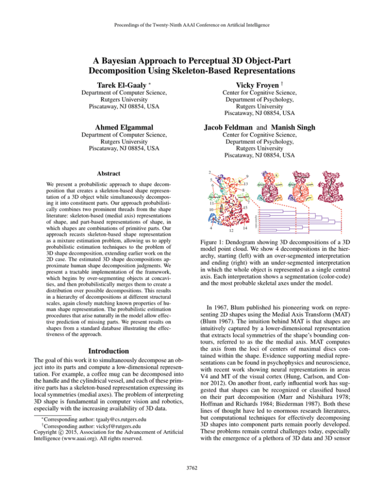
Figure 1: Dendogram showing 3D decompositions of a 3D
model point cloud. We show 4 decompositions in the hierarchy, starting (left) with an over-segmented interpretation
and ending (right) with an under-segmented interpretation
in which the whole object is represented as a single central
axis. Each interpretation shows a segmentation (color-code)
and the most probable skeletal axes under the model.
In 1967, Blum published his pioneering work on representing 2D shapes using the Medial Axis Transform (MAT)
(Blum 1967). The intuition behind MAT is that shapes are
intuitively captured by a lower-dimensional representation
that extracts local symmetries of the shape’s bounding contours, referred to as the the medial axis. MAT computes
the axis from the loci of centers of maximal discs contained within the shape. Evidence supporting medial representations can be found in psychophysics and neuroscience,
with recent work showing neural representations in areas
V4 and MT of the visual cortex (Hung, Carlson, and Connor 2012). On another front, early influential work has suggested that shapes can be recognized or classified based
on their part decomposition (Marr and Nishihara 1978;
Hoffman and Richards 1984; Biederman 1987). Both these
lines of thought have led to enormous research literatures,
but computational techniques for effectively decomposing
3D shapes into component parts remain poorly developed.
These problems remain central challenges today, especially
with the emergence of a plethora of 3D data and 3D sensor
Introduction
The goal of this work it to simultaneously decompose an object into its parts and compute a low-dimensional representation. For example, a coffee mug can be decomposed into
the handle and the cylindrical vessel, and each of these primitive parts has a skeleton-based representation expressing its
local symmetries (medial axes). The problem of interpreting
3D shape is fundamental in computer vision and robotics,
especially with the increasing availability of 3D data.
∗
Corresponding author: tgaaly@cs.rutgers.edu
Corresponding author: vickyf@rutgers.edu
c 2015, Association for the Advancement of Artificial
Copyright Intelligence (www.aaai.org). All rights reserved.
†
3762
a Rotational Symmetry Axis (ROSA) which captures local symmetry of the object shape. The latter approach improves upon this by creating an L1-median skeleton which
locally adapts to the shape. There are many more previous
approaches that fit skeletons to 3D object models, discussed
further in Huang et al. (2013). Although these approaches
are able to find 3D skeletons, they do so using a large set of
free parameters, and are not able to assign graded beliefs to
different possible decomposition interpretations.
One study (Ning et al. 2010) approaches the problem
from a cognitive perspective by first decomposing objects
into parts using segmentation and then computing critical/inflection points based on surface concavities. Skeletons
are then extracted from segmented parts by joining them and
refining the skeleton to represent the topology of the shape
in accordance with Morse Theory (the basis for Reeb Graphs
1D skeletons and analyzing the topology of shapes using
critical points). The emphasis in this approach on critical
points and inflections reflects the prominent role they play in
human shape representation (Winter and Wagemans 2006).
However, in part because of its reliance on critical points, the
method tends to fail in the presence of occlusion, though the
human system can accommodate missing data with relative
ease.
One approach that extracts 2D medial representations
from 3D is Miklos, Giesen, and Pauly (2010). This approach, named the Discrete Scale Axis, improves upon
Blum’s original MAT for 3D objects by following the medial axis transform with topology-preserving angle filtering.
Similarly, Siddiqi et al. (2008) proposed an algorithm for
jointly computing the medial surfaces and object segmentations, resulting in a representation that yields favorable retrieval performance for rigid objects. The problem with 2D
medial representations from a Computer Vision perspective
(i.e for object recognition/matching) is that 2D skeletal representation (e.g. sheets) is still relatively high dimensional.
In Miklos, Giesen, and Pauly (2010) an example of this is
the body of the dolphin which is represented by a relatively
vertical sheet. This seems unnecessary for tubular shapes. A
sufficient representation can be a curve going through the
center of the dolphin’s body with some definition of the
cross-sectional variation along the main axis as in Biederman’s definitions of 3D object parts (Biederman 1987). Despite this, some more rectangular objects require 2D representations, such as sheets.
Several approaches that focus on 3D mesh segmentation
have achieved good performance on the Princeton Benchmark for 3D Mesh Segmentation (Chen, Golovinskiy, and
Funkhouser 2009) and some also represent shapes using
skeletons (Shapira, Shamir, and Cohen-Or 2008; Wong et
al. 2014). Most of these approaches depend on the number
segments/parts k being set prior to decomposition, except
Core Extraction and Shape Diameter Function. The former
decomposes an object hierarchically with a focus on pose
invariance using feature points. No notion of probability
is defined to identify more probable or intuitive decompositions and this method does not use skeletons to achieve
the decomposition. The latter approach is similar to our
approach. The authors jointly decompose objects and re-
applications.
We present a probabilistic model of object-part decomposition and skeletonization of 3D objects. The contributions
of this work are as follows. First, we present a probabilistic estimation procedure for 3D skeleton-based representations of point clouds. Second, simultaneously, our method
decomposes an object into intuitively distinct parts. Third,
our model allows us to assign degrees of belief (probabilities) to distinct part decomposition interpretations. Fourth,
the model provides hierarchical interpretations, providing
not just a single interpretation but a family of possible interpretations at different levels of abstraction, along with a
probability distribution over them. This accords with characteristics of human perceptual organization, and moreover
allows the computational system to interpret objects at multiple scales. Finally, the probabilistic nature of the model allows it to identify both the most probable object decomposition hypothesis and a distribution over a set of alternative
hypotheses.
Related Work
Siddiqi and Pizer (2008) survey the many advances in shape
representation since Blum. They divide shape understanding methods into several types, including landmark representations, boundary representations, displacement by voxel
representations and medial representations. By far the most
popular and intuitive shape representation is the medial representation. Numerous extension and improvements to the
MAT have been proposed, including shock graphs (Macrini
et al. 2002), reeb graphs (Biasotti et al. 2008), flux graphs
(Rezanejad and Siddiqi 2013), object cores (Burbeck and
Pizer 1995), multi-scale medial axes (Pizer et al. 1994),
Bone graphs (Macrini et al. 2011), Bayesian estimation of
the shape skeleton for 2D shapes (Feldman and Singh 2006;
Froyen 2014). Problems with ligatures, noise, missing shape
information due to occlusion and ambiguity in the final representation haunt many of these models because they inherit
the basic limitations of Blum’s approach (Rezanejad and
Siddiqi 2013; Sebastian, Klein, and Kimia 2004). Improvements have been made by either smoothing over the object’s
shape before fitting the skeleton or smoothing the skeletal
representation after fitting. A discussion of these methods
appears in Miklos, Giesen, and Pauly (2010).
Most research on shape, including work nominally oriented towards the 2D case, takes the interpretation of 3D
shape as the more fundamental problem (Hummel and Biederman 1992; Edelman 1997; Hummel and Stankiewicz
1998; Marr and Nishihara 1978; Feldman et al. 2013). Much
of this work focuses on decomposition of shape into primitive parts that are not explicitly medial, and are applied to
hand-crafted 3D objects rather than point-cloud data.
More recently, the Computer Graphics community has explored geometric methods for fitting skeletons to 3D shapes.
The goal is to use these models to perform shape modelling
and analysis for Computer Graphics applications. Two recent methods, Tagliasacchi, Zhang, and Cohen-Or (2009)
and Huang et al. (2013), compute skeletons on incomplete
and initially unorganized point clouds. The former computes
3763
cover the skeleton using a probabilistic membership function (i.e. membership of a vertex into one of the object clusters/parts). The method performs well on articulated objects,
but has trouble with non-articulated objects. Many of the
aforementioned methods suffer from the same limitations
as the traditional MAT approach, which stem from their inherently deterministic nature. Only a small number of approaches aim to estimate medial representations probabilistically. One example of this is Froyen (2014) who assumes
that the underlying skeleton is the generating source of the
point-cloud. A probabilistic estimation procedure enables
these approaches to handle noisy and missing information,
assign beliefs to different decomposition interpretations, incorporate prior knowledge, and predict missing information.
These approaches are, however, confined to 2D shapes, and
probabilistic approaches have not yet been applied to the 3D
case.
Figure 2: Over-Segmentation results for arbitrary large k
values. Notice concavities on the surface of the objects constitute good cut boundaries.
additional cue in determining most-probable merges in the
hierarchy. The normalized cut values are equal to the normalized sum of weights on edges of optimal cuts. We scale
these optimal cuts in the 0-1 range and combine them with
the posterior probabilities of merging two segments. This is
described further in the Hierarchical Grouping section.
3D Perceptual Object-Part Decomposition
Generative 3D Skeletal Representation
In this section we describe our 3D object-part decomposition approach. It is based on the idea that 3D object-part
decomposition can be understood as a Bayesian mixture estimation problem. We propose a tractable implementation
of this framework, which begins by over-segmenting objects at shape concavities, and then probabilistically merging
them into a hierarchical representation, creating a distribution over possible decompositions.
Our approach is based on a framework found in Froyen
(2014) for perceptual grouping in general, and 2D partdecomposition specifically, called Bayesian Hierarchical
Grouping (BHG). This framework has been shown to make
qualitative and quantitative predictions of human behavior
across several areas of perceptual grouping, including 2D
part-decomposition. Here we apply the framework to the
realm of 3D object decomposition with some novel extensions.
Initial Over-Segmentation
The smallest unit of data we consider in this work is a segment of 3D points extracted by Over-Segmentation. In order to find these segments we use Normalized Cuts (Shi
and Malik 2000), similar to Karpathy, Miller, and Fei-Fei
(2013), that prefer segment cuts that lie along concavities. This mimics human perception as humans perceive
part boundaries to be concave while the individual parts of
the object tend to be convex (Hoffman and Richards 1984;
Karpathy, Miller, and Fei-Fei 2013).
Our approach is set up such that Normalized Cuts computes the minimal cuts in the graph connecting the 3D points
of the point cloud. The graph edges are assigned weights
based on angles between neighboring points’ surface normals as follows:
e−α(ni ·(pj −pi ))/2σ
wij =
dij
Mixture Model Within BHG each possible part decomposition interpretation cj ∈ C = {c1 . . . cJ } of a set of
3D points D = {x1 . . . xN } is associated with a posterior
probability p(C|D), which according to Bayes rule is proportional to the product of a prior probability p(C) and a
likelihood p(D|C). Here a decomposition hypothesis cj is a
vector of labels cj = {c1 . . . cN } assigning each set of 3D
points xn to a part m. By adopting the BHG framework, both
the 3D part decomposition problem and 3D skeletonization
can be viewed as a mixture estimation problem. We assume
that the configuration of 3D points making up a 3D shape is
generated by a mixture of M underlying skeletal axes:
p(xn |φ) =
(1)
M
X
p(xn |θm )p(cn = m|p)
(2)
m=1
where cn ∈ c = {c1 . . . cN } are the assignments of data to
an axis, p is a parameter vector of a multinomial distribution
with p(cn = m|p) = pm , θm are the parameters of the m-th
axis, and φ = {θ1 , . . . , θM , p}. Since the problem of estimating mixture consists of estimating which axis m owns
which point xn and the parameters θ of the underlying axes,
both the decomposition problem and the 3D skeletonization
problem are solved in tandem.
where i is the subscript for the central point and j is for the
neighbors of point pi . n are the normals of the corresponding
points and dij is the Euclidean distance between the points.
When angles between ni and (pj −pi ) are > 90◦ , this means
that the surface is convex. The weights in equation 1 are
larger for more convex surfaces. Additionally, we penalize
concavities by using a large α value when the angle is < 90◦
and using a small α for convex angles > 90◦ . This ensures
that optimal cuts are along surface concavities.
The segments found in this way, shown in Fig. 2, serve
as the basic building blocks in our hierarchical approach below and in addition we use the normalized cut values as an
Generative Function The generative function p(xn |θm )
depicting how 3D points are generated from an underlying
axis generalizes the skeletal generating function proposed in
3764
This equation is maximized as a function of q, by means
of a 2-step algorithm (for details see Flöry, 2005). In step 1
the footpoints tn for each point xn is computed. Given these
pairs [xn , tn ], in step 2, we maximize the above equation
using Simulated Annealing (Kirkpatrick, Gelatt, and Vecchi
1983). Both steps are then repeated until convergence. In this
way we not only find an at least locally optimal skeletal axis
representation for a point cloud segment, but also (as incorporated in p(Dm |θ)) we capture how ”part-like” the segment
is, given our prior assumptions.
Our approach should be formulated to be independent
of any user-specified M components. To ensure independence, a Dirichlet process prior is used, as in Froyen (2014),
over the decomposition hypotheses p(cj |α). In this way
the above mixture model becomes a Dirichlet process mixture model which is a widely used non-parametric approach
(Neal 2000). This results in the following definition of the
above introduced posterior for a decomposition hypothesis:
Figure 3: Two cuts showing our 3D generative function. Red
line depicts the underlying B-spline axis. The gradient depicts the probability p(xn |θ), where red has a higher probability.
Feldman and Singh (2006) and Froyen (2014). A flexible
way of representing (and encoding) axes is by means of a
3D parametric B-spline curve gm (t) (Fig. 3), governed by a
parameter vector qm . From this curve data points are generated from a univariate Gaussian distribution perpendicular
to the curve,
p(xn |θm ) = N (dn |am tn + bm , σm )
p(cj |D, α, β) ∝ p(cj |α)
M
Y
p(Dm |β),
(4)
m=1
where dn = ||xn − gm (n)||, called the riblength, is the distance between the datapoint xn and its perpendicular projection on the curve gm (n), referred to as the footpoint.
The mean of the normal distribution is defined as a linear
function of the footpoint positions tn , with slope am , intercept bm and σm is variance over the riblengths (Fig. 3).
Together parameter vector for the generative function becomes θm = {am , bm , σm , qm }. Note that the generative
function constrains parts to obey a kind of local symmetry,
and the linear function over riblengths allows us to capture
conic parts.
In keeping with a full-fledged Bayesian approach a set
of priors over the generative function’s parameters θm is defined, summarized by p(θ|β). Two priors are introduced over
the curve gm itself: one over the squared arclengthF1m of
the curve gm , F1m ∼ exp(λ1 ) and one over the squared total curvature F2m of the curve gm , F2m ∼ exp(λ1 ) , both
respectively governing the elastic and bending energy of the
curve. Lastly, a conjugate prior to the normal distribution is
adopted. The prior over the variance σ is σ ∼ X −∈ (σ0 , ν0 ),
where σ0 depicts the mean variance of the riblength, and ν0
how strongly we believe this. The slope a and intercept b
both have a Gaussian prior distribution, a ∼ N (µ0 , κ−1
0 )
and b ∼ N (µ0 , κ−1
).
Thus
the
hyperparameter
vector
is
de0
fined as β = {µ0 , κ0 , σ0 , ν0 , λ1 , λ2 }
In order to compute the likelihood of a particular decomposition hypothesis p(D|cj ), it is important to integrate over
the axis parameters θ forR each axis, resulting in the marginal
likelihood p(Dm |β) = p(Dm |θ)p(θ|β)dθ, where Dm are
all the points xn belonging to axis cn = m. Unfortunately
integrating over all possible curves (i.e. the parameter space
of qm ) is computationally expensive. The marginal is approximated by only integrating over the Gaussian components, which due to the conjugate formulation can be done
analytically, and selecting qm as to maximize,
Z Y
p(Dm |β, q) =
p(xn |a, b, σ)p(θ|β)dadbdσ. (3)
where M now
R denotes the number of axis specific to cj , and
p(cj |α) = p(cj |p)p(p|α)dp is a standard Dirichlet integral. Unfortunately the size of the hypothesis space C is exponential in the number of 3D points, N . The BHG framework approximates this large posterior, by implementing a
version of the Bayesian Hierarchical Clustering algorithm
by Heller and Ghahramani (2005). Moreover, this approach
results in an intuitive hierarchical representation of the configuration of 3D points.
Hierarchical Grouping
Bayesian hierarchical clustering (Heller and Ghahramani
2005) follows the same concept as traditional Agglomerative clustering algorithms, with the main difference that a
Bayesian hypothesis test is used to decide which clusters to
merge. Here we will briefly sketch the algorithm; for more
details we refer to Heller and Ghahramani (2005). In our
implementation the algorithm will initiate with K trees Tk
each containing the set of 3D points Dk belonging to the kth initial segment as found by the over-segmentation stage
(see above and Fig. 1). At each iteration the algorithm decides which pair of trees (Ti and Tj ) are most likely to be
merged using a Bayesian hypothesis test, resulting in a new
tree Ti∪j containing the data Di∪j = Di ∪ Dj . The pairs of
segment regions of the point cloud are considered for merging if they are adjacent to each other in Euclidean space.
This is a simple way of drastically reducing the complexity
of the computation, since not all pairs must be considered.
In order to compute the likelihood of a merge, two hypothesis are compared. The first hypothesis Hmerge , treats
all data Di∪j as generated from one underlying axis, and can
thus readily be computed as p(Di∪j |Hmerge ) = p(Di∪j |β)
(see Eq. 3). We also benefit from information from the oversegmentation phase which is in the form of the cut values between neighboring segments. We take the product
log p(Di∪j |β) = Cut(Di , Dj ) log p(Di∪j |β) as our new
cn =m
3765
marginal likelihood (adding to Eq. 3). This affects the probability of merging by preferring merges with high cut-values
(i.e. less concavity between the segments).
The second hypothesis Hnomerge , treats all data Di∪j as
generated by more than one axis as constrained by the tree
structure. Its probability is computed by taking the product
over the subtrees p(Di∪j |Hnomerge ) = p(Di |Ti )p(Dj |Tj ).
Here p(Di |Dj ) is computed recursively as the tree is built:
with zero-mean and standard deviation equal to 10-20% of
the mean inter-point distance of neighboring points. As the
noise increases we still obtain a relatively intuitive decomposition.
To validate the generative capability of our model on 3D
data, we show how it performs in reverse by generating the
input data. Fig. 5 and Fig. 6 show the original subsampled
input point cloud with sampled points from our underlying
generative model overlaid. Figure 6 is particularly interesting. We remove a hole in the surface of the Martini Glass
model and are able to reconstruct it by filling it up with
points sampled from the Gaussian distribution of our underlying generative model.
p(Di∪j |Ti∪j ) = p(Hmerge )p(Di∪j |Hmerge )+
(1 − p(Hmerge ))p(Di |Ti )p(Dj |Tj )
where p(Hmerge ) is based on the Dirichlet process prior and
is also computed recursively as the tree is built. The probability of a pair Di and Dj being merged is:
p(Di∪j |Hmerge )p(Hmerge )
p(Di∪j |Ti∪j )
The pair with the highest probability of the merge hypothesis is then merged. In this way the algorithm continues to
greedily build the tree until all data is merged into one tree.
Note that each level along the tree depicts a different decomposition hypothesis (see Fig. 1). The probability of each of
these hypotheses is easily computed using Eq. 4.
ri∪j =
Experimental Discussion
Figure 5: Black points are the subsampled input point cloud
which is used to estimate the underlying generative model.
Red points show sampled points from our underlying probabilistic model (the more opaque being more probable - best
viewed using zoom).
We experimented on the 3D Dataset from Chen, Golovinskiy, and Funkhouser (2009), which provides a large dataset
of 3D meshes - 380 objects across 19 different categories.
We subsample the 3D meshes and reduce the representation
to unorganized 3D point clouds. Each point has its corresponding computed surface normal which is used in oversegmentation. We uniformly subsample the point clouds,
substantially reducing the number of points.
Figure 6: This figure shows the ability to predict missing
data. Here a hole is cut into the side of object and it is filled
by sampling from the underlying generative model. The heat
map depicts the probability of that sample (with red being
higher probability)
Figure 4: Added zero-mean Gaussian noise to one of the airplane object models. Despite noise of up 20% of the mean
inter-point distance, the skeletonization and decomposition
works well.
Figure 1 shows the hierarchical decomposition of a Teddy
Bear. The two center decompositions shown correspond to
local maxima of the posterior probability in the hierarchy.
We find these to be among the most intuitive decompositions. Our maximum-a-posterior (MAP) decomposition is
the second one from the right and corresponds exactly to
14 human annotated teddy bears. This particular object may
be considered an “easy” example but more complex objects
can be seen in Fig. 7 and some of their corresponding human
segmented counterparts in Fig. 8.
We show that our object representations are somewhat robust to noise as shown in Fig. 4. We added Gaussian noise
Conclusion
We have presented a novel procedure for estimating skeletal representations from 3D point clouds and decomposing
them into intuitive component parts. We produce an intuitive
hierarchical tree of abstractions and a distribution over them.
These multiple representations of an object closely match
known properties of human shape representation. We validate this by an experimental study as well as the capability
of dealing with noise and predicting missing data which can
occur due to occlusion.
3766
Figure 7: MAP object-part decomposition for a broad selection of 3D object models. The black curves in each colored segmented represents the estimated skeletal axis of that segment. Notice, for example, the ability to discriminate the 3 parts of the
Martini glass. Notice also the ability to decompose both articulated and non-articulated objects. Some failure cases can be seen
in (d). One or two problematic merges happen due to the non-symmetric torso. Despite this, the skeleton is not compromised.
Figure 8: For comparison, these are a selection of 4 manually human segmented objects. Each object in the dataset has annotations corresponding to, on average, 11 human subject segmentations. MAP decompositions computed by our approach are
shown in the red squares.
3767
Acknowledgments
Kirkpatrick, S.; Gelatt, C. D.; and Vecchi, M. P. 1983. Optimization by simulated annealing. Science 220(4598):671–
680.
Macrini, D.; Shokoufandeh, A.; Dickinson, S. J.; Siddiqi, K.;
and Zucker, S. W. 2002. View-based 3-d object recognition
using shock graphs. In ICPR.
Macrini, D.; Dickinson, S. J.; Fleet, D. J.; and Siddiqi, K.
2011. Bone graphs: Medial shape parsing and abstraction.
Computer Vision and Image Understanding 115(7):1044–
1061.
Marr, D., and Nishihara, H. K. 1978. Representation and
recognition of the spatial organization of three-dimensional
shapes. Proceedings of the Royal Society of London
200(1140):269–294.
Miklos, B.; Giesen, J.; and Pauly, M. 2010. Discrete scale
axis representations for 3d geometry. In SIGGRAPH.
Neal, R. M. 2000. Markov chain sampling methods for
dirichlet process mixture models. Journal of computational
and graphical statistics 9(2):249–265.
Ning, X.; Li, E.; Zhang, X.; and Wang, Y. 2010. Shape decomposition and understanding of point cloud objects based
on perceptual information. In SIGGRAPH.
Pizer, S. M.; Burbeck, C. A.; Coggins, J. M.; Fritsch, D. S.;
and Morse, B. S. 1994. Object shape before boundary shape:
Scale-space medial axes. Journal of Mathematical Imaging
and Vision 4(3):303–313.
Rezanejad, M., and Siddiqi, K. 2013. Flux graphs for
2D shape analysis. In Dickinson, S., and Pizlo, Z., eds.,
Shape perception in human and computer vision, Advances
in Computer vision and pattern recognition. Springer.
Sebastian, T. B.; Klein, P. N.; and Kimia, B. B. 2004. Recognition of shapes by editing their shock graphs. In PAMI.
Shapira, L.; Shamir, A.; and Cohen-Or, D. 2008. Consistent mesh partitioning and skeletonisation using the shape
diameter function. Visual Computation 24(4):249–259.
Shi, J., and Malik, J. 2000. Normalized cuts and image
segmentation. In PAMI.
Siddiqi, K., and Pizer, S. 2008. Medial Representations:
Mathematics, Algorithms and Applications. Springer Publishing Company, Incorporated.
Siddiqi, K.; Zhang, J.; Macrini, D.; Shokoufandeh, A.;
Bouix, S.; and Dickinson, S. 2008. Retrieving articulated
3-d models using medial surfaces. Machine vision and applications 19(4):261–275.
Tagliasacchi, A.; Zhang, H.; and Cohen-Or, D. 2009. Curve
skeleton extraction from incomplete point cloud. In SIGGRAPH.
Winter, J. D., and Wagemans, J. 2006. Segmentation of object outlines into parts: A large-scale integrative study. Cognition 99(3):275–325.
Wong, S.-K.; Yang, J.-A.; Ho, T.-C.; and Chuang, J.-H.
2014. A skeleton-based approach for consistent segmentation transfer. Journal of information science and engineering 30(4):1053–1070.
The research was supported by NSF 1218872 and 1409683
to AE, and NIH EY021494 to JF and MS. The authors would
like to thank Brian McMahan for motivating and helpful discussions.
References
Biasotti, S.; Giorgi, D.; Spagnuolo, M.; and Falcidieno, B.
2008. Reeb graphs for shape analysis and applications. Theoretical Computer Science 392(1):5–22.
Biederman, I. 1987. Recognition-by-components: A theory of human image understanding. Psychological Review
94(2):115–147.
Blum, H. 1967. A transformation for extracting new descriptors of shape. In Models for the Perception of Speech
and Visual Form.
Burbeck, C. A., and Pizer, S. M. 1995. Object representation by cores: Identifying and representing primitive spatial
regions. Vision Research 35(13):1917–1930.
Chen, X.; Golovinskiy, A.; and Funkhouser, T. 2009. A
benchmark for 3D mesh segmentation. In SIGGRAPH.
Edelman, S. 1997. Computational theories of object recognition. Trends in Cognitive Science 8(1):296–304.
Feldman, J., and Singh, M. 2006. Bayesian estimation of
the shape skeleton. Proceedings of the National Academy of
Sciences 103(47):18014–18019.
Feldman, J.; Singh, M.; Briscoe, E.; Froyen, V.; Kim, S.;
and Wilder, J. 2013. An integrated bayesian approach to
shape representation and perceptual organization. In Dickinson, S., and Pizlo, Z., eds., Shape perception in human and
computer vision, Advances in Computer vision and pattern
recognition. Springer.
Flöry, S. 2005. Fitting B-spline curves to point clouds in the
presence of obstacles. Master’s thesis, TU Wien.
Froyen, V. 2014. Bayesian Mixture Estimation For Perceptual Grouping. Ph.D. Dissertation, Rutgers, The State
University of New Jersey.
Heller, K., and Ghahramani, Z. 2005. Bayesian hierarchical
clustering. In ICML.
Hoffman, D. D., and Richards, W. A. 1984. Parts of recognition. Cognition 18(1):65–96.
Huang, H.; Wu, S.; Cohen-Or, D.; Gong, M.; Zhang, H.; Li,
G.; and B.Chen. 2013. L1-medial skeleton of point cloud.
In SIGGRAPH.
Hummel, J. E., and Biederman, I. 1992. Dynamic binding
in a neural network for shape recognition. Psychological
Review 99(3):480–517.
Hummel, J. E., and Stankiewicz, B. J. 1998. Two roles for
attention in shape perception: A structural description model
of visual scrutiny. Visual Cognition 5:49–79.
Hung, C.-C.; Carlson, E. T.; and Connor, C. E. 2012. Medial
axis shape coding in macaque inferotemporal cortex. Neuron 74(6):1099–1113.
Karpathy, A.; Miller, S.; and Fei-Fei, L. 2013. Object discovery in 3d scenes via shape analysis. In ICRA.
3768
