Proceedings of the Twenty-Fifth AAAI Conference on Artificial Intelligence
Markov Logic Sets: Towards Lifted Information
Retrieval Using PageRank and Label Propagation
Marion Neumann and Babak Ahmadi and Kristian Kersting
Knowledge Dicovery Department, Fraunhofer IAIS
53754 Sankt Augustin, Germany
{firstname.lastname}@iais.fraunhofer.de
and in turn can provide useful information as to the features which are relevant for forming that cluster, Ghahramani and Heller (2005) have called it clustering on demand.
More formally, consider a universe of items I. For instance,
I may consist of publications, web pages, images, movies,
places and artifacts found in Pompeii, or any other type of
objects we may wish to form queries on. The user provides a query in the form of a very small subset of items
Q ⊂ I constituting examples of some concept in the data,
say {isa(taberna), city(pompeii)}. The algorithm then
has to provide a completion to the set Q, that is, some set
C ⊂ I that presumably includes all the elements in Q and
other elements in I, which are also elements of this concept,
say {house(h1), house(h2), house(h4), . . .} and other objects that are related to shops in Pompeii.
“GoogleTM Sets” treats the clustering on demand problem as a large-scale clustering problem that involves many
millions of data instances extracted from web data. Ghahramani and Heller (2005) have proposed a Bayesian approach,
called Bayesian sets (BSets), for solving it. As in other
retrieval problems, BSets computes a score measuring for
each item how relevant it is to the query. Specifically, using
a probabilistic model of the unknown concept, it computes
the relevance score by comparing the posterior probability
of an item, given the query, to the prior probability of that
item. However, “GoogleTM Sets” and BSets have focused
on propositional universes assuming that the items are representable as attribute-value vectors. Nowadays, the role of
structure and relations in the data, becomes more and more
important (Getoor and Taskar 2007): information about one
item can help us to draw conclusions about other items.
Such domains are hard to represent meaningfully using a set
of propositional features. Thus, it is natural to ask the question “How do we solve the clustering on demand problem
for relational domains?” An investigation of this question
leads to our main contribution: Markov logic sets (MLS).
Defining the relevance score between two nodes is one of
the fundamental building blocks in graph mining. One very
successful technique is based on random walks with restart
(RWR). Concretely, MLS employs the seminal PageRank
(PR) algorithm (Brin and Page 2006), which is the (limit)
stationary probability that a random walker is at some node,
but personalized on the query. Following the idea underlying BSets, MLS actually computes the relevance score by
Abstract
Inspired by “GoogleTM Sets” and Bayesian sets, we
consider the problem of retrieving complex objects and
relations among them, i.e., ground atoms from a logical
concept, given a query consisting of a few atoms from
that concept. We formulate this as a within-network
relational learning problem using few labels only and
describe an algorithm that ranks atoms using a score
based on random walks with restart (RWR): the probability that a random surfer hits an atom starting from
the query atoms. Specifically, we compute an initial
ranking using personalized PageRank. Then, we find
paths of atoms that are connected via their arguments,
variablize the ground atoms in each path, in order to
create features for the query. These features are used to
re-personalize the original RWR and to finally compute
the set completion, based on Label Propagation. Moreover, we exploit that RWR techniques can naturally be
lifted and show that lifted inference for label propagation is possible. We evaluate our algorithm on a realworld relational dataset by finding completions of sets
of objects describing the Roman city of Pompeii. We
compare to Bayesian sets and show that our approach
gives very reasonable set completions.
Introduction
Imagine you catch parts of a conversation of two archaeologists: “... the room is a taberna ... City of Pompeii ...” What
is the conversation about? Which concept is described by
isa(taberna) and city(pompeii)? “Taberna” is the Latin
word for “shop”, and Pompeii is the Roman city in southern
Italy that was covered in volcanic ash during the eruption of
Mt. Vesuvius in 79 AD. So, the two archaeologists might
have talked about the daily life of Romans in Pompeii and
where they went shopping.
This example encapsulates the very practical and interesting machine learning and information retrieval problem,
namely to automatically create sets/clusters of items from
a few examples only, and has originally been addressed
by “GoogleTM Sets”1 . Since it involves forming a cluster once some elements of that cluster have been revealed
c 2011, Association for the Advancement of Artificial
Copyright Intelligence (www.aaai.org). All rights reserved.
1
http://labs.google.com/sets
447
isa
room
house
0.12
r1
0.13
h1
−0.04
ty1
0.38
t
room
house
0.12
r2
0.12
r4
0.13
h2
room
0.13
h4
0.38
p
−0.51
type
f1
−0.53
r3
house
tasks such as link prediction and entity resolution. Here, we
demonstrate its potential for another important AI and novel
lifted inference task: information retrieval using LP.
We start off by touching upon related work. After reviewing relational logic, pathfinding, and RWR, we develop
MLS. Before concluding, we present our experiments.
isa
room
−0.06
h3
house
city
Related Work
Similar to (Silva et al. 2010), MLS considers the clustering
on demand problem as within-network relational learning
problem: the input is a single data graph in which some of
the instances are labeled and the task is to infer the labels
of the remaining instances, see e.g. (Neville and Gallagher
2009) and references in there. Existing within-network relational learning methods indeed exploit the statistical dependencies among instances in order to improve classification performance. However, they assume that positive and
negative labels are given for some nodes, and inference is
generally still at the level of propositional logic. The latter
also holds for the relational variants of BSets (Silva et al.
2010) and it is difficult — if not impossible — to employ
existing lifted inference for them. Moreover they assume
a single, finite feature space for all items; MLS does not
since it employs RWR and learns query specific features automatically. Lao and Cohen (2010) present an approach to
relational retrieval based on path-constrained RWR; MLS,
however, constructs positive and negative labels from logical features and apllies LP. Muggleton (1996) has proposed
inductive logic programming (ILP) techniques for singlepredicate learning from positive examples only; MLS solves
a multi-predicate learning problem in a transductive setting. Probabilistic Explanation Based Learning (Kimmig,
De Raedt, and Toivonen 2007) produces generalized explanations from examples; MLS can also provide set completions, even if no concept/explanation is present.
Relational pathfinding has been proven successful
for learning the structure of Markov logic networks
(MLN) (Richardson and Domingos 2006). For instance,
Mihalkova and Mooney (2007) as well as Kok and Domingos (2009) proposed to use it to find a path of ground atoms
in the training data. They also variablize ground atoms in the
path but then they construct a MLN whose formulas are the
paths viewed as Boolean variables (conjunctions of atoms).
In contrast, MLS uses the features to compute a PR that generalizes well across similar items.
Finally, MLS is related to recent lifted probabilistic inference approaches traditionally designed for discrete domains, e.g. (Milch et al. 2008). LP, however, requires to
deal with continuous domains. Only very recently, Choi and
Amir (2010) have presented the first continuous lifted variable elimination. Arguably, the simplest and most efficient
approximate lifted inference algorithms are based on the already mentioned LBP approaches. They have been developed for discrete domains only. Only recently, we have developed a lifted GaBP (Ahmadi, Kersting, and Sanner 2011)
and present its first application to clustering here.
To summarize, lifted clustering on demand of arbitrary
relational domains has not been addressed so far.
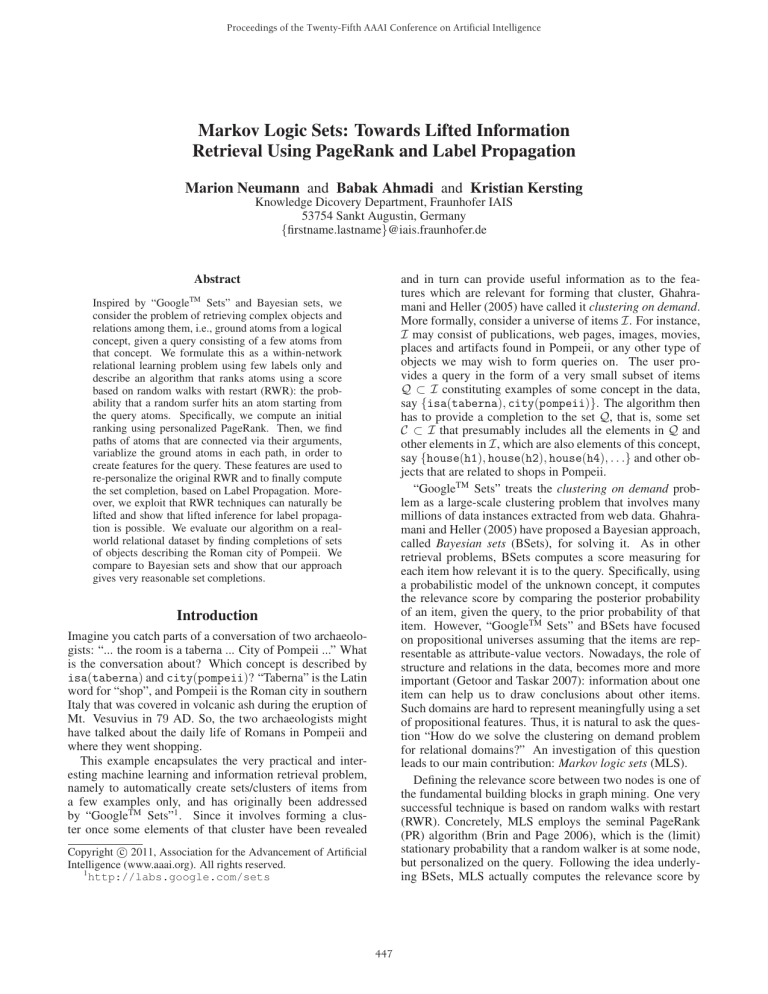
Figure 1: Markov logic sets’ ranking (rounded to the second digit) for the query {isa(taberna), city(pompeii)}
on the toy version of the Pompeii dataset, which is described
in the main text. All houses with a shop are ranked high,
whereas h3 , which has no shop, is ranked low.
comparing the posterior PR of an item given the query, i.e.,
the personalized PageRank, to the prior PR of that item, i.e.,
the uniform PageRank. This differential PR (DPR) has been
proven to be successful for ranking folksonomies (Hotho et
al. 2006) but has two major drawbacks for our setting:
1. It does not make use of the rich structure provided by relational domains. It treats items, i.e., ground atoms monolithically. To generalize across items, we find paths of
ground atoms that are connected via their arguments and
variablize the ground atoms in each path, in order to create
logical features, and use the features to compute a personalization vector for (D)PR.
2. It ranks items high that are generally surprising but unrelated to the query. To overcome this, we only estimate
negative (positive) labels for items ranked lowest (highest) by DPR if they conform the features. Then, the labels
are spread across the graph using label propagation (LP),
see e.g. (Zhou et al. 2003), another RWR technique.
We evaluate MLS2 by finding completions of sets of realworld objects describing the Roman city of Pompeii. For
instance, MLS discovers that the two archaeologists talked
about “shopping places in Pompeii” as shown in Fig. 1. A
comparison to BSets using our logical features shows that
MLS give very reasonable set completions.
However, this paper makes another important and novel
contribution. We note that the core computations in both
PR and LP, namely solving systems of linear equations
can be done distributively and efficiently using Gaussian
belief propagation (GaBP), see e.g. (Shental et al. 2008).
There are, however, many improvements that can be made
to (Ga)BP, especially when applied to inference in graphical
models containing structural symmetries. Such symmetries
are commonly found in relational domains. To exploit these
symmetries, lifted BP (LBP) approaches have been recently
developed (Singla and Domingos 2008; Kersting, Ahmadi,
and Natarajan 2009) to automatically group nodes and potentials together into supernodes and superpotentials if they
send and receive identical messages. LBP then runs a modified BP on this lifted network. LBP has been proven to yield
significant efficiency gains compared to BP on important AI
2
The use of Markov random walks as well as logical features to
compute set completions also explains the name Markov logic sets.
448
Relational Logic and Pathfinding
Algorithm 1: Markov Logic Sets
Input: Query set Q, Graph G = (V, E)
1 Set V+ = Q and V− = ∅ /* Initialize labels */;
2 Set L = ∅ /* Initialize feature set */;
3 xq = PPR(G, Q) /* PPR on Q*/ ;
4 Compute paths P in G (up to depth k) that start in one
of the query atoms in Q;
5 foreach p ∈ P do /* Pathfeatures */
6
Generalize p into pathfeatures F by variablizing
some of the arguments /* see main text */;
7 foreach f ∈ F do /* Logical features */
8
if f is discriminative then /* see main text */
9
Include f in L;
In relational logic, see e.g. (De Raedt 2008), formulas
are constructed using three types of symbols: constants,
variables, and predicates. Constants represent objects in
a domain of discourse (e.g., houses such as h1 , h2 , etc.,
cities such as pompeii, and rooms such as r1 , r2 , etc.
Variables (e.g., uppercase X, Y) range over the objects.
Predicates represent relations among objects (e.g., in(h1 , p)
and in(r1 , h1 )), or attributes of objects (e.g., isa(r1 , t)
where t denotes taberna). An atom is a predicate symbol
applied to a list of arguments, which may be variables
or constants (e.g., in(X, p)). A ground atom is an atom
all of whose arguments are constants (e.g., in(h1 , p)).
A universe is a set of ground atoms. As an example,
consider the following universe over objects in the city
of p, houses h1 ,h2 , h3 ,h4 , rooms r1 ,r2 ,r3 ,r4 , functions of
rooms t, f1 , and room types ty1 : {in(h1 , p), in(h2 , p),
in(h3 , p), in(h4 , p),in(r1 , h1 ), in(r2 , h2 ), in(r3 , h3 ),
in(r4 , h4 ), isa(r1 , t),isa(r2 , t), isa(r4 , t), isa(r3 , f1 ),
typeof(r3 , ty1 ),
typeof(r1 , ty1 ),typeof(r2 , ty1 ),
typeof(r4 , ty1 )}, which is motivated by a real-world
database3 of objects found in Pompeii (Allison 2001).
A universe can be viewed as a hypergraph. A hypergraph
is a straightforward generalization of a graph, in which an
edge can link any number of nodes, rather than just two.
More formally, a hypergraph is a pair (V, E) where V is a set
of nodes, and E is a multiset of labeled non-empty subsets
of V , called hyperedges. Now, the constants appearing in a
universe are the nodes and ground atoms are the hyperedges.
Each hyperedge is labeled with the predicate symbol of the
corresponding ground atoms. Nodes (constants) are linked
by a hyperedge if and only if they appear as arguments in
the hyperedge. Examples are shown in Fig. 2 where we have
omitted the edge labels but have associated the type of nodes
for the sake of readability.
In MLS, we find paths in a hypergraph corresponding to a
universe. A path is defined as a set of hyperedges such that
for any two hyperedges e0 and en in the set, there exists an
ordering of (a subset of) hyperedges in the set e0 , e1 , . . . , en
such that ei and ei+1 share at least one node. A path of hyperedges can be generalized into path features, i.e., conjunctions of relational atoms by variablizing their arguments.
10
11
12
13
14
15
16
17
18
19
20
21
22
23
24
xp = PPR(G, w) /* reweighted PPR */ ;
xu = PR(G) /* uniform PR */ ;
xd = xp − xu /* differential PR */ ;
foreach v ∈ V do /* Label Set */
Add v to V− if |xi (v) − min xi | < , i ∈ {p, d} and
no ground feature fired for v;
Add v to V+ if |xi (v) − max {xi (u)|u ∈ Q}| < ,
i ∈ {p, d} and a feature fired for v;
Run LP on G using V+ and V− as pos resp. neg labels;
Return the ranking r produced by LP;
positive and negative labels for some of the nodes of the
graph, we can employ another RWR technique, called label
propagation (LP), to propagate the information through the
graph in order to label all unlabeled nodes, see e.g. (Zhou
et al. 2003). We compute the diagonal degree matrix D
with Dii =
j Aij . Then, we compute the normalized
graph Laplacian L = D−1/2 AD−1/2 , and initialize a column vector y according to the labels we have, that is yi = 1
if node i is labeled positive, yi = −1 if labeled negative,
and yi = 0 otherwise. The final labeling x can then be computed by solving the following system of linear equations
(I − αL)x = (1 − α)y. We note that the core computations in both PR and LP can be solved by combining Shental
et al.’s (2008) GaBP approach to solving linear systems together with Kersting, Ahmadi, and Natarajan’s (2009) color
passing approach for LBP, yielding Lifted GaBP (LGaBP).
(Lifted) Random Walk with Restarts
Recall the RWR approach to ranking nodes in a graph
touched upon in the introduction. In a nutshell, a Markov
chain transition matrix M is constructed out of a given
graph G. Let A be the m × m adjacency matrix of G, that is
Aij = 1 if there is an edge from vertex j to vertex i and zero
otherwise. PageRank (PR) now constructs the probability
transition matrix M by adding 1T to all 0T rows and renormalizes each row of A to sum up to 1. Furthermore, a prior
probability v can be taken to weight the results. The personalized PR (PPR) can then be computed by solving the following system of linear equations (I − αMT )x = v where
α trades off speed of convergence with the accuracy of the
solution and I is the identity matrix. If we additionally have
3
foreach v ∈ V do /* Reweighted Personalization */
w(v) = 0 /* weight of item v */ ;
foreach matching of l ∈ L in G ending in v do
Let xq (f, v) be the PPR of the item matching
the end atom of l;
w(v) = w(v) + xq (f, v);
Markov Logic Sets
Alg. 1 summarizes MLS, and Fig. 2 provides an example
run with query {house(h1 ), house(h2 )} for the universe of
objects in the city of Pompeii described previously.
MLS begins with computing the PPR on the query Q
(line 3). The result, see Fig 2(a), illustrates that this PPR
is not enough to solve the clustering on demand problem.
http://www.stoa.org/projects/ph/home
449
isa
room 0.44
r1
house
0.26 type
ty1
0.23
t
1.00
h1
room 0.44
r2
house
1.00
h2
0.00
isa
f1
0.11 room
r3
0.15 room
r4
0.16
house
h4
isa
0.15
house
h3
room 0.00
r1
house
0.00 type
ty1
0.46
t
2.00
h1
room 0.00
r2
house
2.00
h2
room 0.42
r1
house
1.00
h1
0.05 type
ty1
room 0.42
r2
house
1.00
h2
0.23 room
r4
0.45
house
h4
0.15
house
h3
0.00 city
p
(a) PageRank xq personalized on Q
0.40
t
0.00 room
r3
0.00 room
r4
0.16
house
h4
0.82 city
p
isa
0.00
isa
f1
(b) (Unnormalized) reweighted personalization w
0.46
isa
f1
isa
0.00 room
r3
room 0.13
r1
0.40
0.41
house house
h3
h1
0.37 city
p
−0.03
type
ty1
0.10
t
room 0.13
r2
house
0.41
h2
0.13 room
r4
−0.52
isa
f1
−0.54
room
r3
−0.08
0.41
house
house
h4
h3
0.28 city
p
(c) Differential PageRank xd = xp − xu
(d) Final LP Ranking r
Figure 2: The major steps of running Markov logic sets for the query {house(h1 ), house(h2 )} on the toy version of the
Pompeii dataset, which is described in the main text. The final ranking is shown in (d). Using 0.0 as threshold would result in
{h1 , h2 , h4 , p, r1 , r2 , r4 , t} as set completion.
House h4 should be in the set completion as it has a shop.
Including also r4 , the room of h4 , also includes h3 , the only
house without a shop. Excluding r4 , however, is suboptimal
as it is the only room and the shop of h4 .
To improve upon this, MLS generalizes the personalization values across the network. Hence, MLS finds paths in
the hypergraph (line 4), say p = “house(h1 ) − in(r1 , h1 ) −
room(r1 ) − typeof(r1 , t) − isa(t)”, and variablizes all
its arguments except the atoms in the start and end nodes.
To create candiate logical features per path the constants in
the start and end nodes are variablized in all possible combinations (lines 5-6), for the example path above, one of the
four possible pathfeatures is: f = “house(X) − in(Y, X) −
room(Y) − typeof(Y, t) − isa(t)”, here only h1 is variablized. However, MLS selects only discriminative features
(lines 7-9). It checks whether (1) the variance of the personalized PageRank scores of query items covered by a feature
(PR presonalized on end atoms) is small and (2) their mean
is significantly different from the mean of PageRank scores
of items over the same predicate that are not in the query
(line 7). Only if (1) and (2) succeed using a χ2 -test, we include the feature (line 9), this applies for example to f .
Afterwards, MLS recomputes the personalization of each
node in G using the resulting logical features, again based
on the PPR on Q (lines 11-15). For our running example,
this yields the unnormalized personalization vector shown
in Fig 2(b). As one can see, the weight of item taberna is
increased from 0.0 (it is not a query member, consequently
its initial personalization was 0.0) to 0.46. One is tempted to
just recompute the PPR using this new personalization, and
indeed items with minimal rank are definitely unrelated to
the query — therefore we give them a negative label (line 21)
but only if no feature fired for the item — and taberna gets
ranked higher now. However, h3 and h4 still get similar, low
relevance score: the concept “houses with shops” has not
been identified yet. Why is this the case?
Ranking items simply by the (reweighted) personalized
PR is not sensible since some items may be more probable
than others, regardless of the query. MLS removes this effect
by computing the differential PR (DPR) w.r.t. to the uniform
PR (lines 17-19). This DPR is shown in Fig 2(c). Now, it is
sensible to assign positive (negative) labels to the items with
maximal (minimal) DPR (lines 20-22) if features have (not)
fired. Finally, MLS runs LP using V+ and V− to create the
final ranking (line 23) as shown in Fig. 2(d). As one can see,
r4 and h3 can clearly be separated.
Experimental Evaluation
Our intention here is to investigate the following questions:
(Q1) Is MLS effective in ranking atoms w.r.t. a given query?
(Q2) How does MLS perform compared to BSets and MLS’s
intermediate rankings xp and xd ? (Q3) Are there symmetries in the LP matrix that can be employed by LGaBP?
To this aim, we implemented MLS and BSets in Python
using LGaBP for the PR and LP computations. In all experiments, we set α = 0.5 for the RWR computations. For
(L)GaBP, we used the “flooding” message protocol where
messages are passed in parallel each step. Messages were
not damped, and the convergence threshold was 10−8 . We
did not compare to Silva et al.’s (2010) relational BSets variant as they assume a single joint feature space. To accom-
450
xp
xd
BSetsF
BSetsL
MLS
xp
xd
BSetsF
BSetsL
MLS
xp
xd
BSetsF
BSetsL
MLS
xp
xd
BSetsF
BSetsL
MLS
Q1 = {house(h2 ), house(h5 ), house(h9 ), house(h12 )}
4 query houses, 1 function, city(pompeii), 3 types, 2 functions, 13 rooms of h2 , 2 types, 1 function, 13 rooms of h5
4 query houses, 13 rooms of h2 , 20 rooms of h5 , 3 rooms of h12 , 4 rooms of h9
all 30 houses, 1 rooms of h2 , 4 rooms of h5 , 2 rooms of h12 , 3 types
8 houses with shops, 11 rooms (shops), isa(taberna), typeof(ty20 ), 19 other houses
typeof(ty20 ), isa(taberna), 8 houses with shops, 22 other houses, city(pompeii), 7 rooms (shops)
Q2 = {house(h2 ), house(h5 ), house(h9 )}
3 query houses, 1 function, city(pompeii), 3 types, 13 rooms of h2 , 1 function, 1 type, 17 rooms of h5
3 query houses, 13 rooms of h2 , 20 rooms of h5 , 4 rooms of h9
3 query houses, all remaining 27 houses, 8 rooms of h2 resp. h5 , 2 types
3 query houses, all remaining 27 houses, 10 rooms
3 types and 3 functions of rooms appearing in the query houses, all 30 houses, city(pompeii), 3 rooms
Q3 = {room(r1e ), room(r1r ), room(r1h ), room(r1f ), room(r1o )}
house(h1 ), 5 query rooms, 4 functions, 5 types, city(pompeii), 15 rooms of h1 , 6 houses, 2 types, 1 function
house(h1 ), 5 query rooms, 15 rooms of h1 , 1 type, 15 functions, 5 other rooms
5 query rooms, 15 rooms of h1 , 20 other rooms
20 rooms of h1 , city(pompeii), house(h1 ), 18 other rooms
house(h1 ), 5 query rooms, 15 rooms of h1 , 3 types resp. functions of rooms in Q3 , city(pompeii), 12 other rooms
Q4 = {p(a1 ), p(a3 ), p(a4 )}
p(a4 ), p(a1 ), p(a3 ), p(a2 ), p(a5 ), p(b5 ), p(d2 ), c(a2 ), s(a2 ), s(a3 ), p(d1 ), p(d3 ), p(b2 ), p(c4 ), p(d4 ), p(d5 ), p(b1 ), p(b4 ), p(b3 ), p(c2 )
p(a3 ), p(a1 ), s(a2 ), s(a1 ), s(a4 ), c(a2 ), c(a4 ), p(a5 ), s(a3 ), p(a4 ), s(b5 ), c(b5 ), s(d2 ), s(b2 ), c(d1 ), c(b1 ), s(b1 ), s(b4 ), p(b3 ), p(d5 )
p(a5 ), p(a3 ), s(a3 ), s(a4 ), s(a2 ), s(a1 ), s(b2 ), s(b4 ), s(b1 ), s(b5 ), s(d2 ), p(a1 ), p(a2 ), c(a2 ), c(a4 ), c(b1 ), c(b5 ), c(d1 ), p(a4 ), p(d5 )
p(a1 ), p(a4 ), p(a2 ), p(a3 ), p(a5 ), s(a4 ), s(a1 ), s(a2 ), s(a3 ), c(a2 ), c(a4 ), c(b1 ), s(b1 ), s(b2 ), s(b4 ), s(b5 ), c(b5 ), s(d2 ), c(d1 ), p(b5 )
p(a5 ), p(a3 ), p(a4 ), p(a1 ), s(a2 ), c(a2 ), p(a2 ), s(a3 ), s(a1 ), s(a4 ), c(a4 ), p(d2 ), s(d2 ), p(d4 ), p(d5 ), p(d1 ), c(d1 ), p(c4 ), p(d3 ), p(c3 )
Table 1: Rankings produced by MLS, intermediate rankings of MLS, and BSets: (Q1 -Q3 ) Top 40 ranked ground atoms
for three different queries on the Pompeii dataset consisting of rooms in 30 Pompeian households. Due to space limitations,
the rankings are shown using a compressed, almost natural language like representation. E.g. “4 query houses, 1 function,
city(pompeii), ...” denotes a ranking in which the four houses in the query are ranked first, followed by a ground atom
describing a function of a room, followed by the ground atom city(pompeii), and so on. (Q4 ) Top 20 ranked ground atoms
for a query consisting of 3 persons from clique a on the smoker-friends graph, where ai denotes the i-th person in clique a.
Predicates are person, cancer, smokes (denoted by p, c and s) and friends. Items of clique a are highlighted.
xp , xd , and BSetsF do not cover the set of houses with
shops and the query relevant information. BSetsL and MLS,
however, are able to retrieve the houses with shops, the respective rooms and their type and function information. In
other words, they have discovered the concept “houses with
shops”. Other houses are also ranked high, since one of the
discriminative features is house(X). By just removing one
house from the query as done in Q2 , the concept “houses
with shops” is not clearly identified by any method. MLS,
though, provides query relevant information such as common discriminative types and functions of the query houses
(isa(taberna), among others). Apart from completing the
set of all houses, it also retrieves city(pompeii). The intermediate MLS rankings fail to return reasonable information
as for example other houses. The third query consisted of 5
out of a total of 20 rooms in house(h1 ). The rankings illustrate that MLS is able to capture all relevant information, by
ranking house(h1 ) the highest followed by all its rooms, the
types and functions of the query atoms and city(pompeii).
BSets as well as xp and xd provide only parts of the information, but no complete summary. The results for query Q4 are
qualitatively similar. In particular, all elements of clique a
are ranked highest only by MLS and BSetsL .
All together, this clearly shows that (Q1) MLS finds reasonable set completions and that (Q2) its performance is better than its intermediate rankings and as good as or even
better than BSets using relational features. The difference
in performances of the two BSets variants demonstrate that
modate for this, we ran BSets (with its parameter c = 2) using our feature sets F resp. L. More precisely, BSetsF uses
all possible relational pathfeatures, whereas BSetsL includes
only the discriminative features found by MLS. For evaluation purposes, we ran all approaches on two datasets: a relational dataset in the spirit of the smoker-friends Markov
logic network and Allison’s (2001) Pompeii dataset mentioned already earlier. Allison has used data about artifacts
in their original context to challenge many common assumptions about the function of particular types of objects, the
use of particular spaces, and the consistency of patterns of
use across different houses. The dataset contains more than
6000 artifact records for finds in 30 architecturally similar
“atrium-style” houses in Pompeii. Artifacts are annotated
with one of 240 typological categories (coin, amphora, etc.)
and in which of the rooms they were found. In total, there
are 863 rooms in the 30 houses. For each room, we have
its type (main garden, front hall, shop, etc.) and function
(culina, taberna, etc.). We have focused on the rooms and
houses providing us with a dataset consisting of 959 node
potentials and 6063 edge potentials (viewed as a graphical
model as used by (L)GaBP). The smoker-friends graph consists of one single connected component of 20 persons of
which 9 smoke and 5 have cancer. That is, we have a total of
34 nodes and 150 edges. There are 4 cliques of friends {a,
b, c, d} with few inter-clique links. Tab. 1 shows the results.
The first query consisted of 4 out of a total of 8 houses
with shops. As one can see the rankings/completions of
451
discriminative relational pathfeatures indeed carry useful information. The compression ratios of the LP matrices – ratio
of (# nodes + # edges) lifted vs. ground – were 0.55 for Q1
- Q3 and 0.73 for Q4 . This shows that (Q3) lifted inference for label propagation is possible and sensible; GaBP
and LGaBP produced the same results.
De Raedt, L. 2008. Logical and Relational Learning.
Springer.
Getoor, L., and Taskar, B., eds. 2007. An Introduction to
Statistical Relational Learning. MIT Press.
Ghahramani, Z., and Heller, K. 2005. Bayesian Sets. In
Proc. Adv. in Neural Inform. Processing Systems (NIPS-05).
Hotho, A.; Jäschke, R.; Schmitz, C.; and Stumme, G. 2006.
Information Retrieval in Folksonomies: Search and Ranking. In Proceedings of the 3rd European Semantic Web Conference (ESWC-06), 411–426.
Kersting, K.; Ahmadi, B.; and Natarajan, S. 2009. Counting
Belief Propagation. In Proceedings of the 25th Conference
on Uncertainty in Artificial Intelligence (UAI–09).
Kimmig, A.; De Raedt, L.; and Toivonen, H. 2007. Probabilistic Explanation Based Learning. In Kok, J. N.; Koronacki, J.; de Mántaras, R. L.; Matwin, S.; Mladenic, D.;
and Skowron, A., eds., ECML, volume 4701 of Lecture
Notes in Computer Science, 176–187. Springer.
Kok, S., and Domingos, P. 2009. Learning Markov Logic
Network Structure via Hypergraph Lifting. In Proc. of the
International Conference on Machine Learning (ICML-09).
Lao, N., and Cohen, W. W. 2010. Relational retrieval using
a combination of path-constrained random walks. Machine
Learning 81(1):53–67.
Mihalkova, L., and Mooney, R. 2007. Bottom-Up Learning
of Markov Logic Network Structure. In Proc. of the Intern.
Conf. on Machine Learning (ICML-07).
Milch, B.; Zettlemoyer, L.; Kersting, K.; Haimes, M.; and
Pack Kaelbling, L. 2008. Lifted Probabilistic Inference with
Counting Formulas. In Proc. of the 23rd AAAI Conf. on
Artificial Intelligence (AAAI-08).
Muggleton, S. 1996. Learning from Positive Data. In
Proceedings of the Inductive Logic Programming Workshop
(ILP-96), 358–376.
Neville, J., and Gallagher, B. 2009. Evaluating Statistical
Tests for Within-Network Classifiers of Relational Data. In
Proc. of the Intern. Conf. on Data Mining (ICDM-09).
Richardson, M., and Domingos, P. 2006. Markov Logic
Networks. Machine Learning 62:107–136.
Shental, O.; Bickson, D.; Siegel, P. H.; Wolf, J. K.; and
Dolev, D. 2008. Gaussian Belief Propagation Solver for
Systems of Linear Equations. In Proc. of the IEEE Int. Symp.
on Inform. Theory (ISIT).
Silva, R.; Heller, K.; Ghahramani, Z.; and Airoldi, E. 2010.
Ranking Relations using Analogies in Biological and Information Networks. Annals of Applied Statistics.
Singla, P., and Domingos, P. 2008. Lifted First-Order Belief
Propagation. In Proc. of the 23rd AAAI Conf. on Artificial
Intelligence (AAAI-08), 1094–1099.
Zhou, D.; Bousquet, O.; Lal, T. N.; Weston, J.; and
Schölkopf, B. 2003. Learning with Local and Global Consistency. In Thrun, S.; Saul, L. K.; and Schölkopf, B., eds.,
NIPS. MIT Press.
Conclusions
We have introduced Markov logic sets (MLS), the first, generally applicable, retrieval framework for relational data that
can naturally be lifted4 . It takes a query consisting of a small
set of ground atoms, and returns additional ground atoms
which belong in this set. Specifically, it computes a relevance score for each ground atom by comparing the personalized PageRank for it given the query, to the unpersonalized PageRank of that ground atom. Since similar items
should intuitively get similar relevance scores, MLS uses relational pathfinding to find generalized personalization vectors. Based on the relevances, positive and negative labels
are constructed that are turned into the final ranking using
(lifted) label propagation. The experimental results demonstrate that lifted retrieval is not insurmountable: MLS performs effectively in retrieving relational set completions.
There are several attractive avenues for future work. We
have not yet addressed in detail how to set the size of the
completion. Since we use LP, using zero as threshold would
be a natural choice but other thresholds are possible. It is
also interesting to apply ILP techniques on the completion
to extract a general description of the latent concept. Using
dynamic PageRank techniques would pave the way to online clustering on demand and is definitely a growth path for
lifted inference. Since lifting of LP itself is an advance, further experimentation and application of lifted inference for
semi-supervised learning is another important direction.
Acknowledgments: The authors thank the anonymous reviewers for their comments. All authors were supported by
the Fraunhofer ATTRACT fellowship STREAM and by the
European Commission under contract number FP7-248258First-MM.
References
Ahmadi, B.; Kersting, K.; and Sanner, S. 2011. MultiEvidence Lifted Message Passing, with Application to
PageRank and the Kalman Filter. In Walsh, T., ed., Proceedings of the 22nd International Joint Conference on Artificial
Intelligence (IJCAI–11).
Allison, P. 2001. Pompeian Households: an Analysis of the
Material Culture. Cotsen Institute of Archaeology.
Brin, S., and Page, L. 2006. The Anatomy of a Large-Scale
Hypertextual Web Search Engine. Computer Networks and
ISDN Systems 30:197–117.
Choi, J., and Amir, E. 2010. Lifted Inference for Relational
Continuous Models. In Proceedings of the 26th Conference
on Uncertainty in Artificial Intelligence (UAI-10).
4
We attempt to develop a pragmatic and general framework that
is liftable; at the moment, we make no claim that lifted techniques
necessarily run faster than a specialized, one-off solution.
452