SIMON FRASER UNIVERSITY
Department of Economics
Econ 808
Macroeconomic Theory
Prof. Kasa
Fall 2005
PROBLEM SET 1 - Time Series and Dynamic Optimization
(Due October 4)
1. Solving the Continuous-Time LQR Three Different Ways
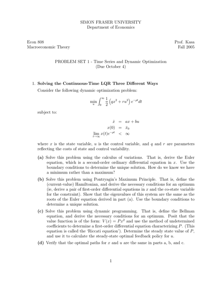
Consider the following dynamic optimization problem:
min
u
∞
0
1 2
qx + ru2 e−ρt dt
2
subject to:
ẋ = ax + bu
x(0) = x̄0
lim x(t)e−ρt < ∞
t→∞
where x is the state variable, u is the control variable, and q and r are parameters
reflecting the costs of state and control variability.
(a) Solve this problem using the calculus of variations. That is, derive the Euler
equation, which is a second-order ordinary differential equation in x. Use the
boundary conditions to determine the unique solution. How do we know we have
a minimum rather than a maximum?
(b) Solve this problem using Pontryagin’s Maximum Principle. That is, define the
(current-value) Hamiltonian, and derive the necessary conditions for an optimum
(ie, derive a pair of first-order differential equations in x and the co-state variable
for the constraint). Show that the eigenvalues of this system are the same as the
roots of the Euler equation derived in part (a). Use the boundary conditions to
determine a unique solution.
(c) Solve this problem using dynamic programming. That is, define the Bellman
equation, and derive the necessary conditions for an optimum. Posit that the
value function is of the form: V (x) = P x2 and use the method of undetermined
coefficients to determine a first-order differential equation characterizing P . (This
equation is called the ‘Riccati equation’). Determine the steady state value of P ,
and use it to calculate the steady-state optimal feedback policy for u.
(d) Verify that the optimal paths for x and u are the same in parts a, b, and c.
1
2. Solving the Discrete-Time LQR Three Different Ways
Consider the following dynamic optimization problem:
min
{ut }
∞
1
β t (qx2t + ru2t )
2 t=0
β<1
subject to:
xt+1 = axt + but
x0 = x̄0
t
lim β xt < ∞
t→∞
where xt is a discrete sequence of state variables, ut is a discrete sequence of control
variables, and q and r are parameters reflecting the costs of state and control variability.
(a) Solve this problem using the calculus of variations. That is, derive the Euler
equation, which is now a second-order (linear) difference equation in xt . Use the
boundary conditions to determine the unique solution.
(b) Solve this problem using the maximum principle, i.e., attach a sequence of Lagrange Multipliers to the constraints. Derive a pair of (linear) first-order difference equations in xt and the Lagrange Multiplier. Show that the eigenvalues of
the first-order system are the same as the roots of the characteristic equation in
part (a). Use the boundary conditions to determine a unique solution.
(c) Solve this problem using dynamic programming. That is, define the Bellman
equation, and use it to characterize an optimal feedback policy for ut . Posit
that the value function is of the form V (xt ) = 12 Pt x2t , and use the method of
undetermined coefficients to calculate a first-order (nonlinear) difference equation
for Pt . (This equation is called the Riccati equation). Prove that there is a unique
positive steady state solution of the Riccati equation.
(d) Verify that the optimal paths for xt and ut are the same in parts a, b, and c.
3. Use the MATLAB program bigshow.m to simulate the following time series processes
and to report their impulse response functions and their (log) spectral densities.
(a) xt = εt
(b) xt = εt + .5εt−1
(c) xt = .9xt−1 + εt
(d) xt = 1.2xt−1 − .3xt−2 + εt
(e) xt = 1.2xt−1 + .3xt−2 + εt
(f) xt = .8xt−1 − .5xt−2 + εt
where εt is an iid shock. Briefly comment on the stochastic properties of these processes.
Which exhibit business cycle features? Which are stationary? Do any possess interior
maxima in their spectral densities? If so, what is the frequency of the implied cycle?
2
4. Do Exercise 2.14 in Ljungqvist & Sargent.
5. Do Exercises 5.1 in Ljungqvist & Sargent.
6. At the beginning of each period, a worker can choose to work at her last period’s wage
or draw a new wage. If she draws a new wage, the old wage is lost and she must wait
one period before she can start her new job. New wages are i.i.d. draws from the c.d.f.
t
F , where F (0) = 0, F (B) = 1 for B < ∞. The worker seeks to maximize E0 ∞
t=0 β wt ,
where wt is the wage in period-t.
(a) Write down the Bellman equation for the worker. (Hint: the value function appears
in both options available to the worker).
(b) Now suppose the worker receives an unemployment compensation of c. What is
the Bellman equation now?
(c) Assume wage offers are distributed uniformly on the interval [0, 1]. Use the program ex2.m to numerically solve the Bellman equation for alternative values of
β and c. (This program first discretizes things and then uses a value function
iteration method. The value function iteration is done by calling the program
valit.m.) How does the reservation wage vary with β and c? Interpret the results.
3