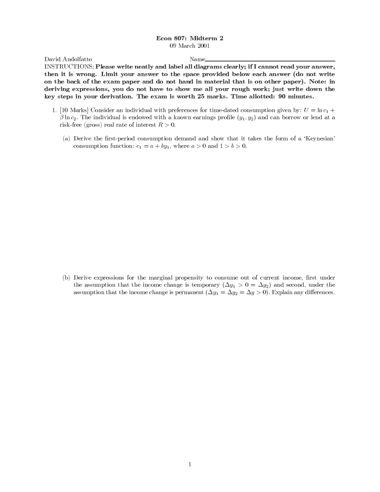
Econ 807: Midterm 2
09 March 2001
Name
David Andolfatto
INSTRUCTIONS: Please write neatly and label all diagrams clearly; if I cannot read your answer,
then it is wrong. Limit your answer to the space provided below each answer (do not write
on the back of the exam paper and do not hand in material that is on other paper). Note: in
deriving expressions, you do not have to show me all your rough work; just write down the
key steps in your derivation. The exam is worth 25 marks. Time allotted: 90 minutes.
1. [10 Marks] Consider an individual with preferences for time-dated consumption given by: U c1
β c2 . The individual is endowed with a known earnings profile y1 , y2 and can borrow or lend at a
risk-free (gross) real rate of interest R > .
(a) Derive the first-period consumption demand and show that it takes the form of a ‘Keynesian’
consumption function: c1 a by1 , where a > and > b > .
= ln
ln
(
+
)
0
=
+
0
1
0
(b) Derive expressions for the marginal propensity to consume out of current income, first under
y2 and second, under the
the assumption that the income change is temporary y1 >
assumption that the income change is permanent y1 y2 y > . Explain any differences.
(∆
(∆
1
= ∆
0 = ∆
= ∆
0)
)
2. [10 Marks] A person has preferences for current and future consumption given by U c1 βc2,
where β > . As well, the person owns and operates a production technology y A k , where A > 0
and k represents capital in place at the beginning of period t. (Assume that k1 is given and that
capital depreciates fully after one period). The productivity parameter A follows a two-state Markov
process; i.e., let Pr[A +1 = A A = A ] = π > 1/2, where A A ,A , A < A .
(a) Let R(A ) denote the (gross) expected return to investment when A = A . Show that R(A ) >
R(A ) and explain.
= ln
0
=
t t
+
t
t
t
j
|
t
j
j
j
∈ {
L
t
H
}
t
L
L
j
H
H
(b) Solve for the optimal investment choice and explain how it depends on the current state of technology A = A (there are two effects to consider: a wealth effect and an expectations effect).
t
j
2
3. [5 Marks] The ‘stimulative’ effects of government spending in a ‘Keynesian’ model.
Now, sit back and relax on this one. This is a question that is designed to teach you the difference
between description (i.e., measurement) and explanation (i.e., theory). Now, we know from our basic income
accounting exercises that one way to measure GDP is to add up the expenditure components; i.e., Y ≡
C + I + G (let’s forget about net exports). This expression is true by definition. Students sometimes
mistakenly reason that, since this expression is true, it must be the case that an increase in G (government
purchases) leads to an increase in GDP. Certainly, we were are all exposed to models (i.e., theories) that
generated such an implication. However, what is important to realize here is that such a prediction cannot
be made solely on the basis of the identity above. In order to make a prediction, one needs a theory and
the identity above is just a way of measuring things—it is not a theory. In order to demonstrate this point,
let me develop a model in which the identity above holds, but nevertheless predicts that an increase in G
results in a decline in Y. Your job is to explain the economic intuition behind this result.
The model is based on the IS-LM-FE analysis that you’ve likely encountered
as an undergrad. Let us
consider
the
labour
market
first.
Labour
supply
is
given
by
a
function
N s(w) and labour demand is given
d
by N (w, R). Here, w represents the real wage and R represents the real interest rate. Assume that labour
supply is increasing in w and that labour demand is decreasing in w. We will also make the assumption
that the demand for labour depends negatively on R (for example, this might be reasonable if the business
sector must borrow funds to finance the period’s wage bill). For a given interest rate R, we can solve for the
market-clearing wage rate by setting N s (w) = N d (w,R). We can denote by N (R), the equilibrium level of
employment conditional on a given interest rate R. Likewise, we can derive an ‘aggregate supply’ function by
inserting N (R) into the business sector’s production function; i.e., Y s (R) = F (N (R)), where F is increasing
in the labour input. Convince yourself that Y s (R) is a decreasing function of R.
Now, let us consider the aggregate demand for output. Consumer demand is given by C d = C0 (a
parameter). Investment demand is given by the function I d (R), which is decreasing in R. The demand for
output from the government sector is given by Gd = G0 (a parameter). Therefore, the aggregate demand
for output is given by Y d (R, C0 ,G0 ) = C0 + I d (R) + G0 . Clearly, Y d is a decreasing function of R and an
increasing function of C0 and G0 . The equilibrium interest rate is given by the R that satisfies the goodsmarket clearing condition: Y s (R) = Y d (R,C0 ,G0 ). It will be helpful for you to draw each of these functions
on a diagram, with Y on the vertical axis and R on the horizontal axis. Assume that the Y s curve is ‘flatter’
than the Y d curve. Show that, for this model, we have Y = C + I + G and dY/dG < 0. What is going on
here?
3